Project
Machine Learning with Regression Models (Part 2)
Part Two
Welcome to Part Two of the Machine Learning activity!
To recap from Machine Learning Pt. 1, up to this point you have done the following:
- Set up your project by downloading the needed code files
- Received a summary of the different Machine Learning modules that will be used in the provided code
- Chose your target trait to be analyzed by the Machine Learning modules
- Prepared the dataset that will be analyzed in this section
- Set up and moved the code files that we will be working with, to Google Colab
Please visit Part One of the Machine Learning activity if you need a recap, or need to review on keep concepts/vocabulary!
SECTION 1
Running the Model and Collecting Outputs
At this point in the Machine Learning activity, we now have our dataset cleaned and your machine learning module/dataset uploaded to Google Colab. Lets start to run the code shall we!
- Your dataset and model notebook should be loaded into Google Colab at this point.
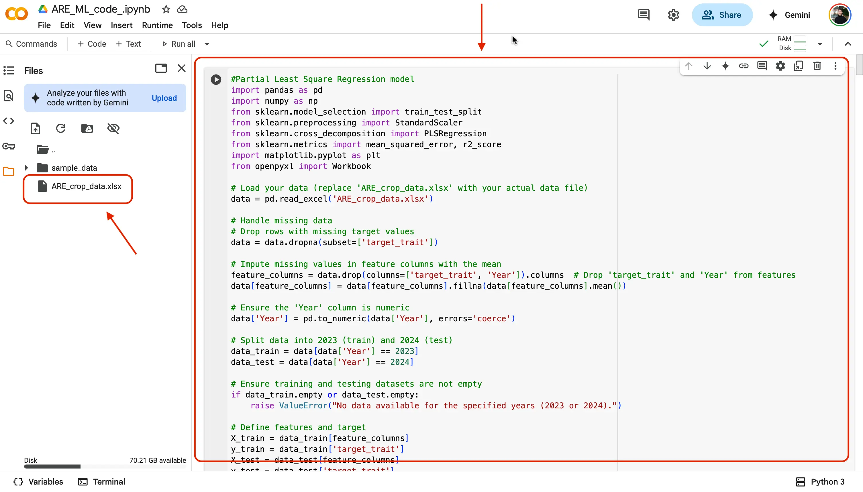
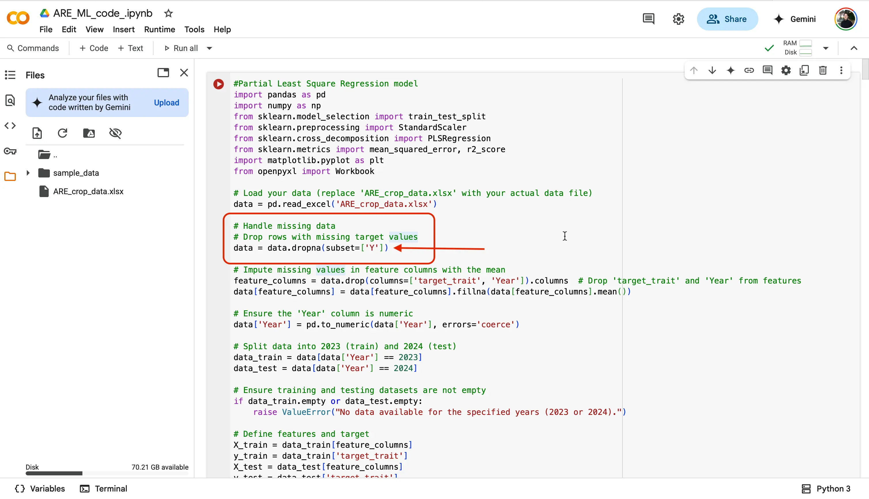
- Lets walk through the first model together! You should see the name of the first model at the very top, "#Partial Least Square Regression model". Notice above the rest of the code is the comments we talked about earlier ( # followed by green text ). At the beginning of the code we are first importing in all of the required python libraries and dependencies needed to make our code work (e.g.,
pandas,numpy,scikit-learn,matplotlib,openpyxl, etc.).
Further Explained
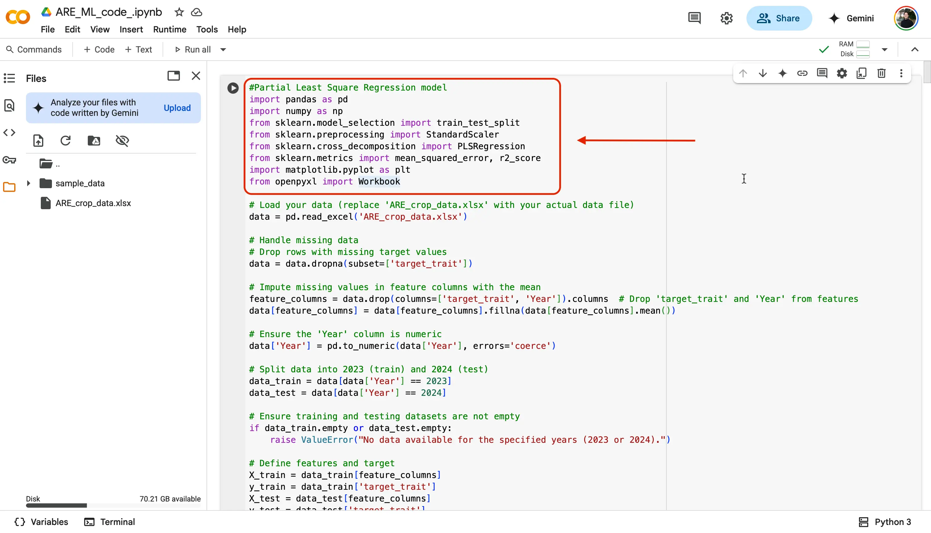
At the beginning of the code, we start by importing all the Python libraries and tools (called dependencies) that we need for our program to work properly. These libraries are like pre-made toolkits that help us do specific tasks easily. For example:
pandashelp us work with tables and spreadsheets (like Excel) in Python,numpylets us do fast math with numbers and arrays,scikit-learnprovides machine learning tools for training and testing models,matplotlibis used to make graphs and visualizationsopenpyxlallows us to read and write Excel files (.xlsx).
By importing these libraries, we don’t have to build everything from scratch, we can just use their built-in functions to make our code shorter, faster, and more powerful!
The next chunk of code is what will be allowing our
ARE_crop_data.xlsxdataset file to be used in our notebook.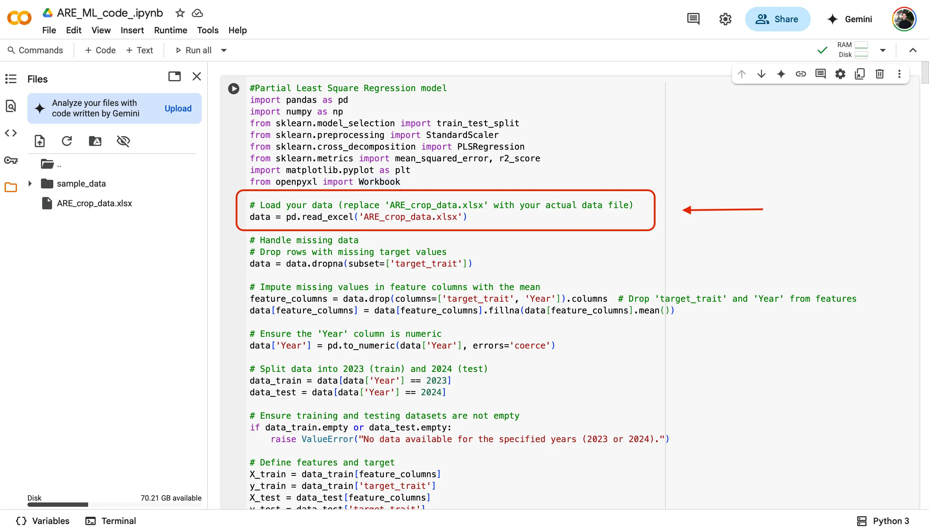
This next code block is very important! This is where you will be choosing your desired trait to analyze from the
ARE_crop_data.xlsxdataset file.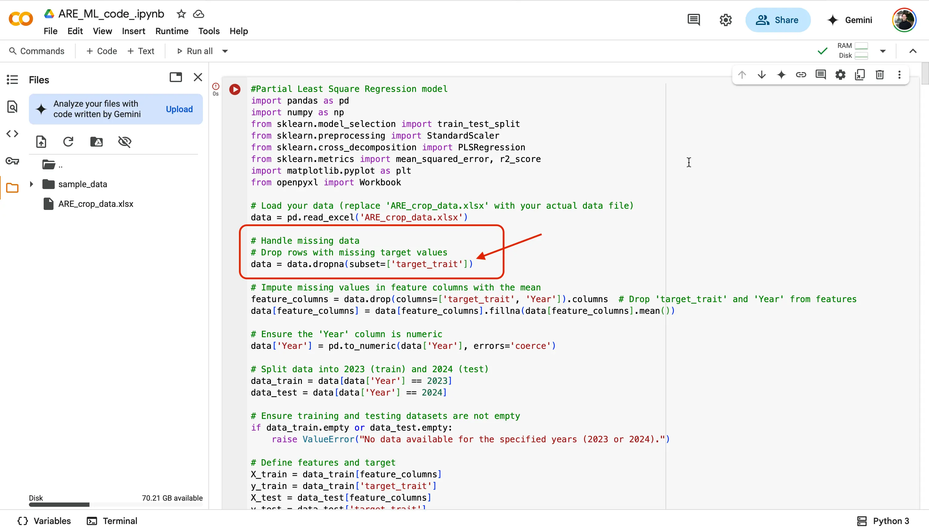
Go back to the
ARE_crop_data.xlsxdataset file, and choose a trait! We are going to chooseYield(Y).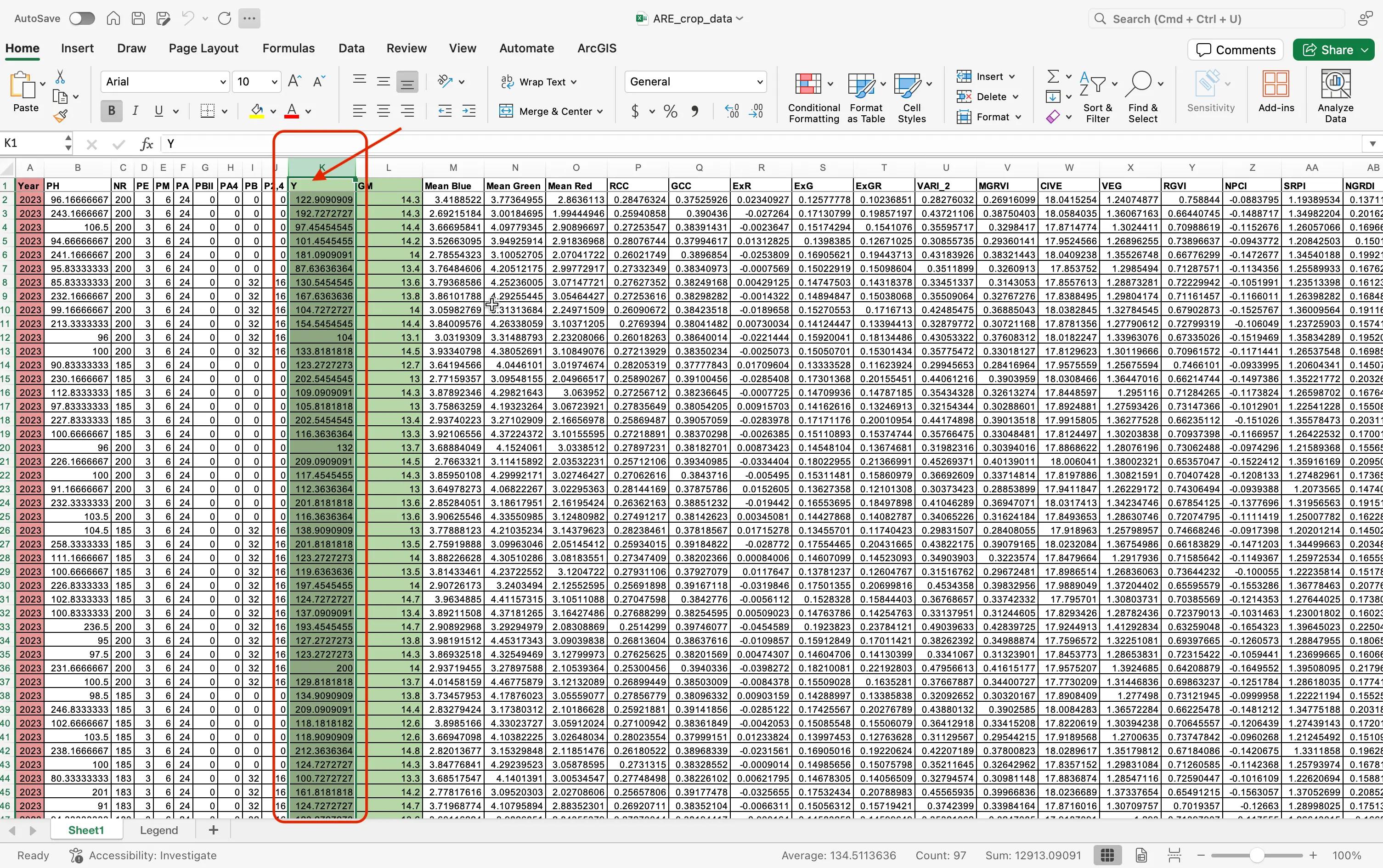
Now since we chose the trait
Yield(Y), we are going to replacetarget_trait, withY.
data = data.dropna(subset=['target_trait'])
To:
data = data.dropna(subset=['Y'])
Important!
We are writing Y and not "Yield" because even though the Y = Yield, in our dataset file the column is strictly labeled as Y only!
- You will now need to update all of the locations that say
target_traittoY.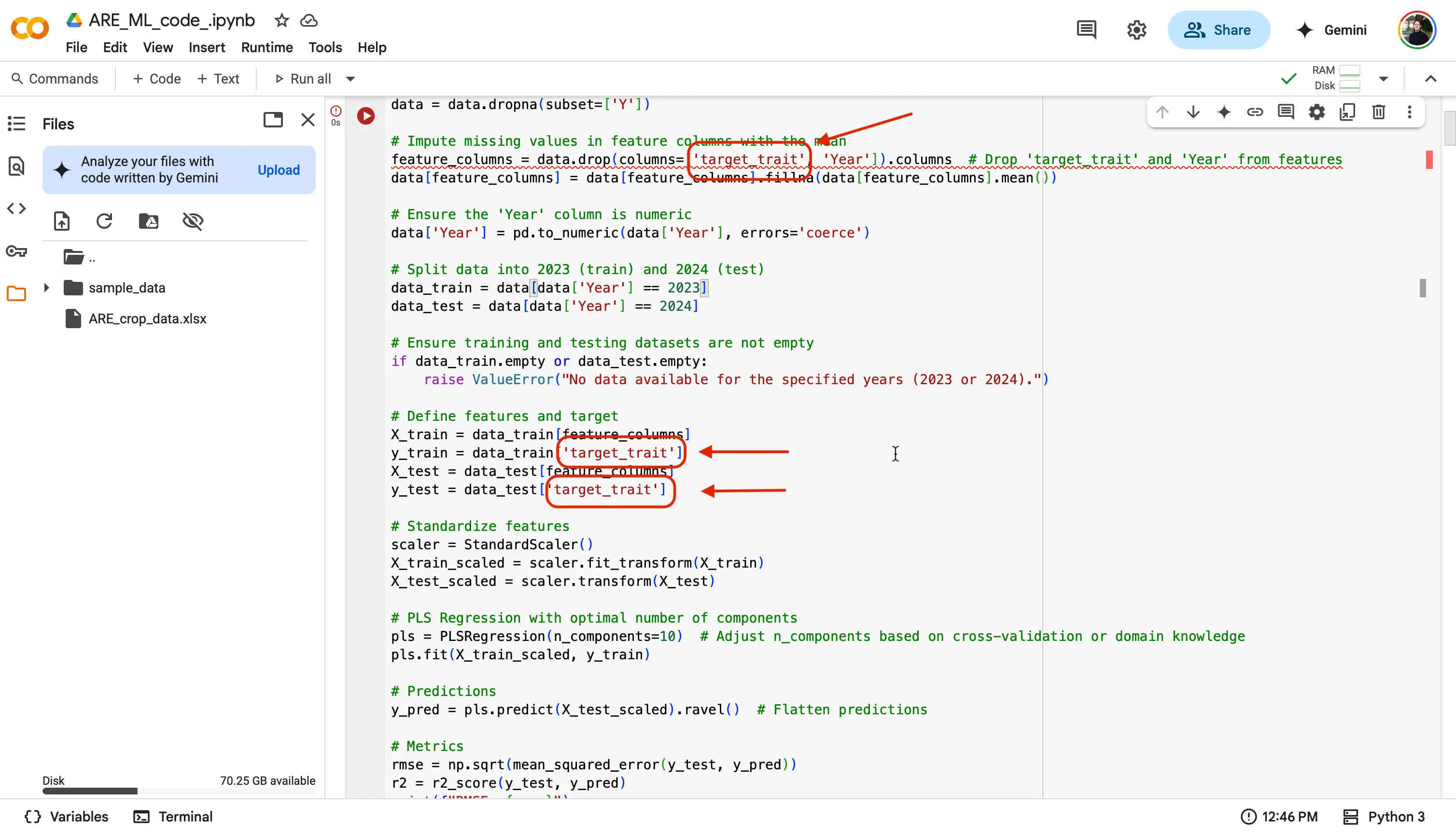
Important!
You will have to do this step for each new model that you start to work on! Whenever you choose a trait, you will have to put that trait, and replace the
target_traitspot in the code. - And that is it! Since you have selected a trait to analyze, and let the code know which trait from the dataset you are looking to analyze, you are good to run the code! We will do this by finding the Play button at the top left of a code block, and selecting it.
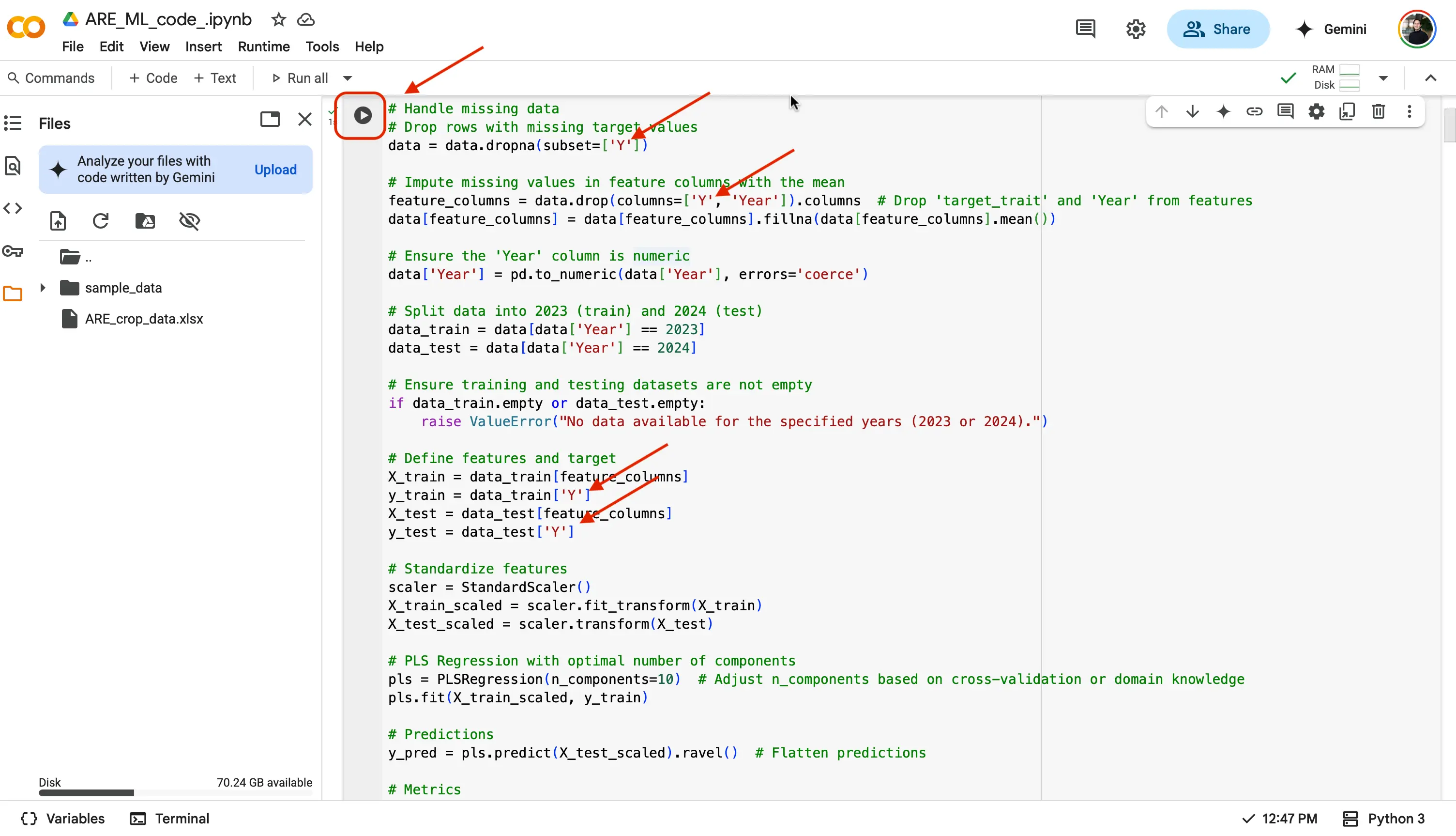
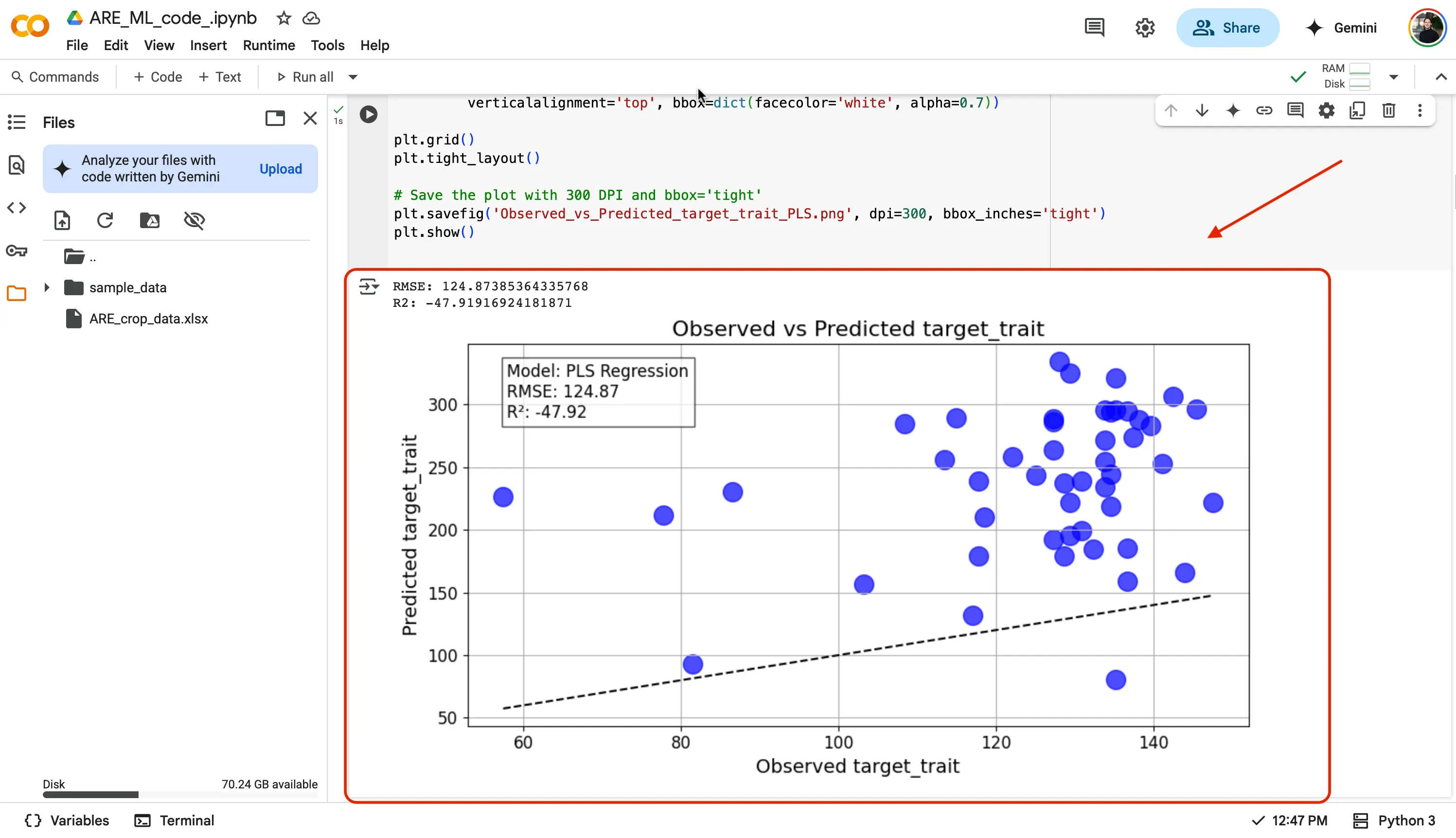
If successfull, you should see a green checkmark next to the play button, and underneath the code:
- A figure showing the regression plot of the predicted vs. observed values.
BREAK!
Lets for a moment, let us break down what we are seeing with our newly created regression plot!
Guidance on How to Read the Observed vs. Predicted Graph
Let’s unpack our regression plot in simple terms.
What you’re looking at:
- A scatterplot where each dot shows one prediction (vertical axis) versus the real value (horizontal axis).
- A perfect model would put every dot right on the diagonal line (45° line) where predicted = actual.
How to tell if it’s good:
- Dots close to the line → small errors (good).
- Dots far from the line → big errors (not so good).
What patterns can tell you:
- If most dots hug the line but some stray far off, your model generally works but makes big mistakes on certain points.
- If dots form a curve or cluster away from the line, your model might be too simple (underfitting) or too tailored to one part of the data (overfitting).
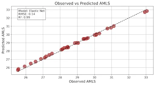
Visual Examples Below:
Here is an example of regression plots you might expect to generate. This graph that you are seeing has very good model output as the R2 is close to 1 and the RMSE is low:
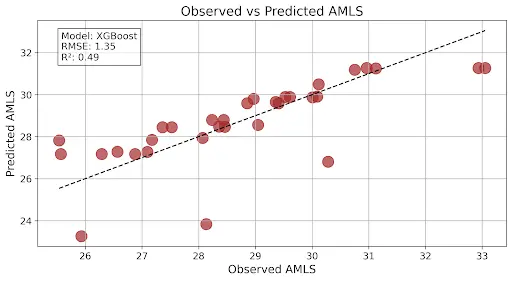
This graph shows a good model output as R2 is a midpoint between 0 and 1 and the RMSE is higher than what the above graph is showing:
Stop & Discuss
Students:
- In one sentence, what does a point far from the diagonal line tell you about the model’s prediction?
- How could you tell from the plot if your model is underfitting or overfitting?
- What would it mean if all points cluster tightly but off the line?
Teachers:
- Ask a student to describe what the diagonal (45°) line represents.
- Invite someone to explain why patterns in the plot (e.g., a curve or fan shape) hint at bias or variance issues.
- Check for any confusion about how the observed vs. predicted plot differs from looking at raw error values.
Stretch break / water break before we start tuning!
In the ARE_ML_code.ipynb file, you might have seen by now that there are other models for you to play with! As a reminder, these other models are:
- Partial Least Squares (PLS) Regression: Finds patterns by combining features into simpler parts to predict something when you have lots of related data.
- Lasso Regression: Helps pick only the most important features by shrinking less useful ones down to zero.
- ElasticNet Regression: Combines Lasso and another method (Ridge) to balance feature selection and avoid overfitting.
- Bayesian Ridge Regression: Adds a bit of randomness to the prediction process to make it more stable and handle uncertainty better.
- Xtreme Gradient Boosting (XGBoost): Builds lots of small decision trees that learn from each other to make powerful predictions.
- Support Vector Regression (SVR): Tries to find a smooth line that fits the data while ignoring small errors, making it good for tricky patterns.
All of these model's code allow you to replace the selected trait. Feel free to now try using your previously selected trait (Y) or a new one, with the other models, to analyze! Let us give you a few examples of different traits you can use:
- Amlysose from starch (AMLS)
- Lysine from grain (LysG)
- Crude Protein (CP)
data = data.dropna(subset=['AMLS'])
or
data = data.dropna(subset=['LysG'])
or
data = data.dropna(subset=['CP'])
Important!
Remember, we wrote Y and not "Yield" because even though Y = Yield, in our dataset file the column is strictly labeled as Y only! Make sure to insert AMLS, LysG, CP, or whatever else you choose.
You should know!
That everytime you run a code block, the graph/figure that you created at the bottom of the code, and an excel file with the Observed and Predicted results will be saved in the console on the left. If you do not see it, you may have to use the refresh button. 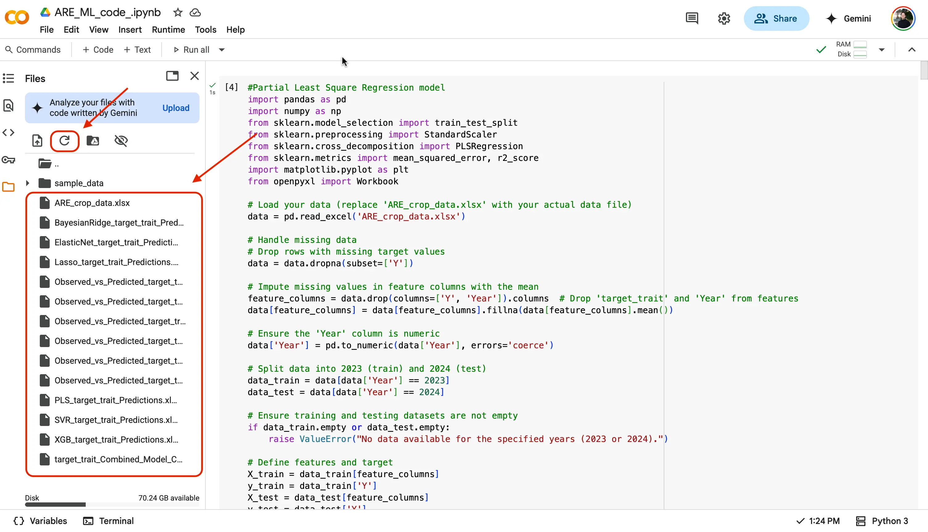
Step by step breakdown of the code blocks
For your reference, here is the breakdown of the summary of each block of code for a model (this is the same information that is in the comments in the green text ). We are just putting this here so you can see a summarized version of each step of the code blocks provided:
- Loading your dataset into your chosen environment (Google Colab).
- Import the necessary libraries (e.g., pandas, numpy, scikit-learn, matplotlib, openpyxl, etc.).
- Loading and handling missing data.
- Spliting your dataset so that data from 2023 is used for training and data from 2024 is used for testing.
- Define features and target
- Transformation and scaling
- Train the models
- Prediction and evaluation
- Save the outputs
SECTION 2
Understanding The Results
When you run the code, you’ll get two main outputs:
A regression plot
- A graph that shows your model’s predictions versus the actual measurements.
An Excel file with two section tabs:
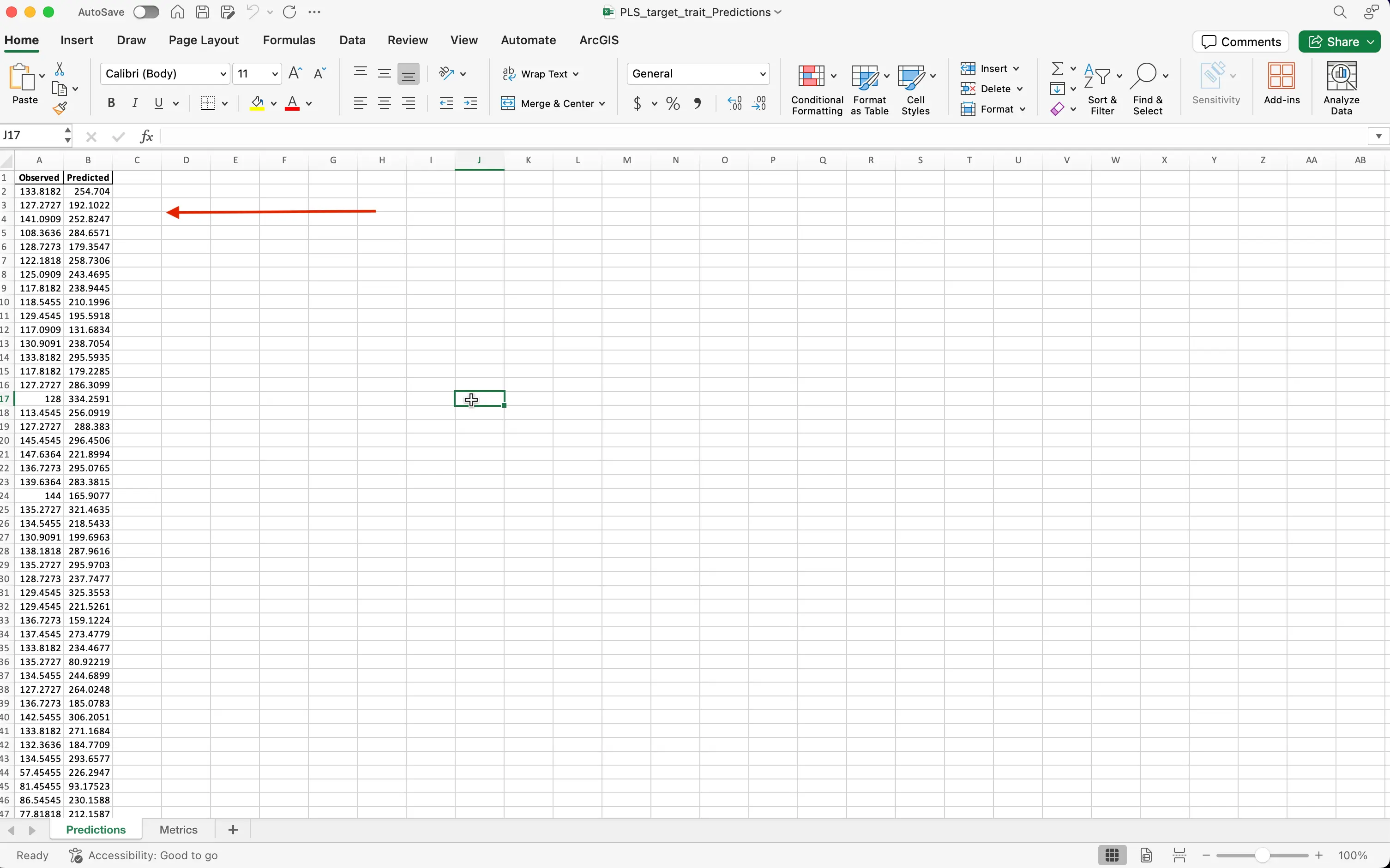
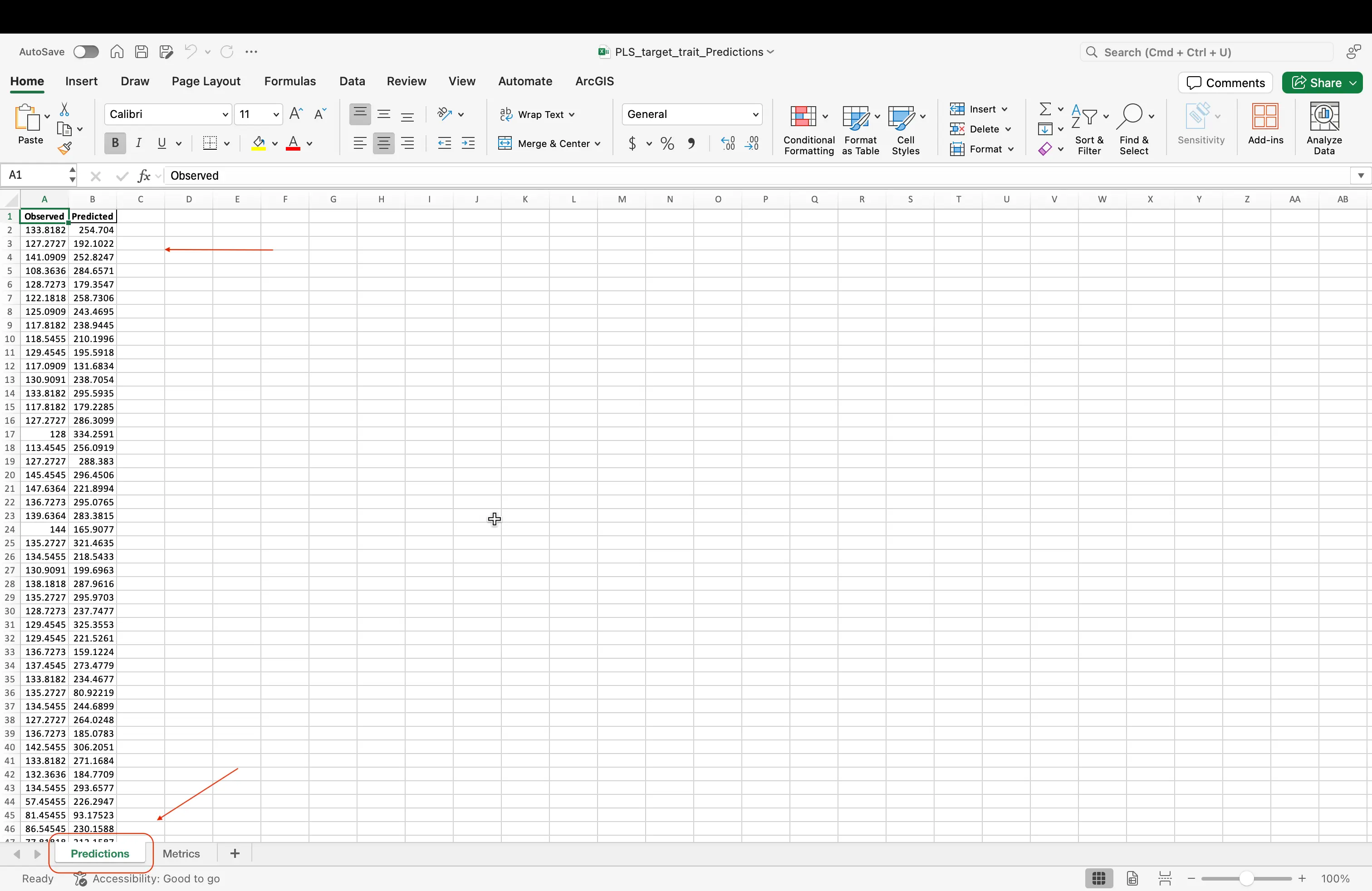
- Observed vs. Predicted values (Predicted tab):
- A side-by-side list of the real measurements from 2024 and the numbers your model (trained on 2023 data) guessed. This shows how well your model works on new data!
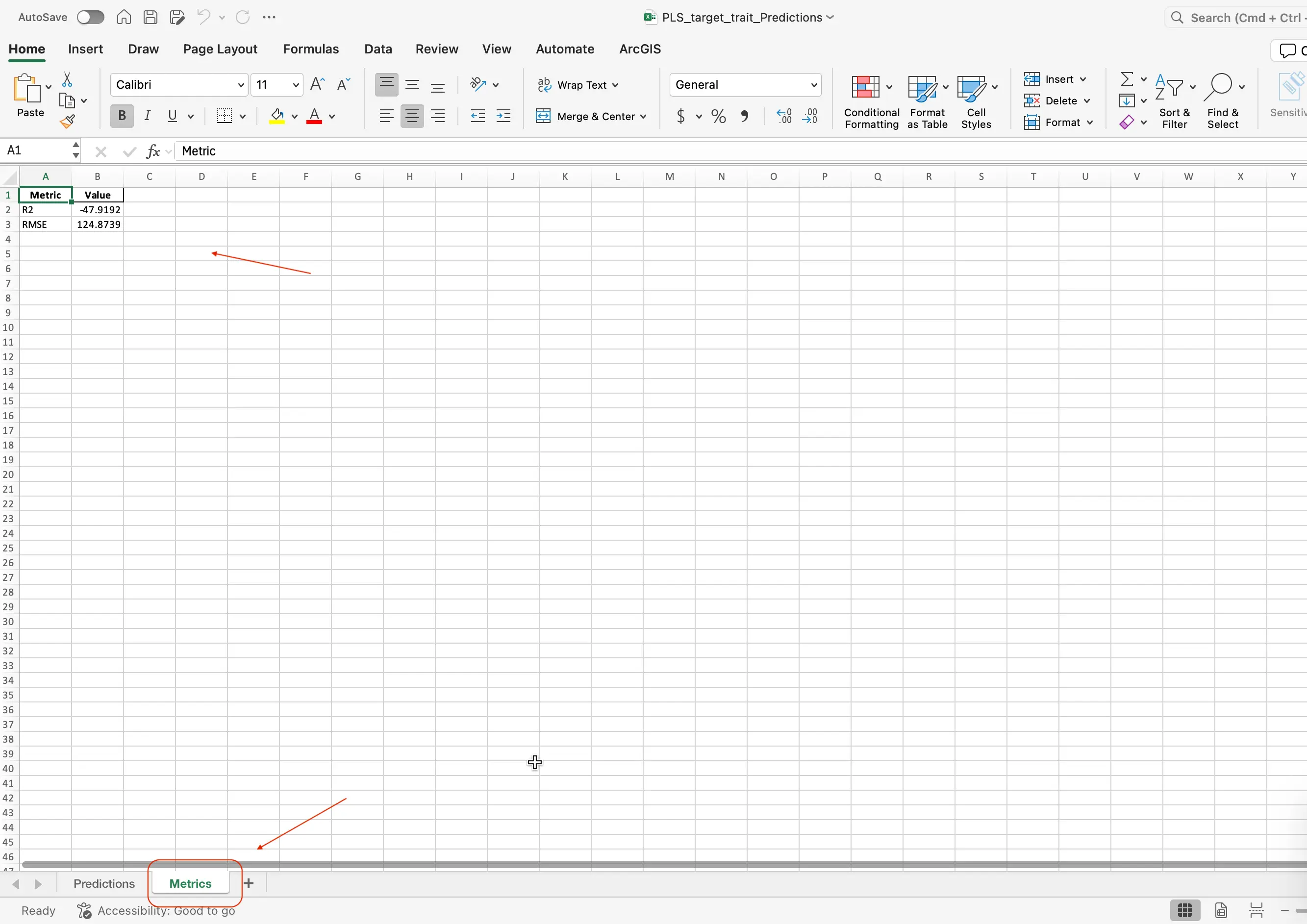
- Metrics (Metrics tab):
- Model scores (R² and RMSE):
- R² tells you what fraction of the real-world variation your model explains (closer to 1 is better).
- RMSE tells you the average size of your model’s mistakes (smaller is better).
- Model scores (R² and RMSE):
Tip: After running all the code blocks, scroll to the bottom of the Excel sheet to find the Predictions and Metrics sections.
You should know!
The Predictions and Metrics values can be found at the bottom of the excel sheet that is outputed to you, once you have ran the code blocks in the exercise. 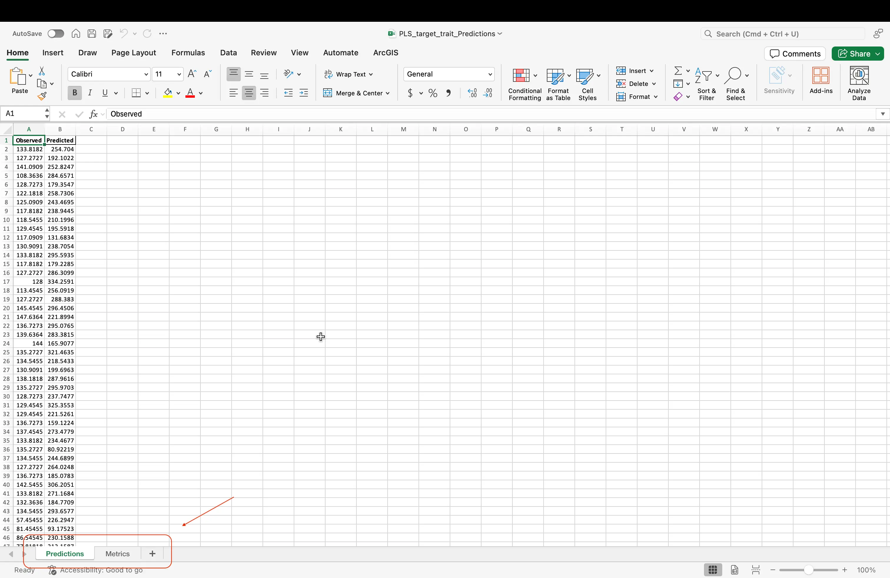
Tuning Your Models
Now that you have your model code complete, the next step would be to tune your model! Tuning a model essentially means tweaking its “settings” (hyperparameters), like how quickly it learns or how complex it is, to get the best accuracy. You do this by testing different combinations (e.g. via cross validation, grid search or cross-validation) and picking the one that makes your predictions most reliable.
Tuning a machine learning model is a pretty complex task, so here’s a more down-to-earth way to think about “tuning” a machine-learning model. Lets imagine for a second that you’re perfecting a cookie recipe:
Adjust your “recipe settings”
- In ML these are called hyperparameters: things like how big a step the model takes when learning (learning rate), how many “mini-models” it builds (number of estimators), or how much it smooths out extreme guesses (regularization strength).
- Real-world example: When baking, you decide how much sugar (learning rate) and how many chocolate chips (estimators) to use. Too much sugar and the cookies burn; too few chips and they’re bland—just like bad hyperparameter choices hurt your model’s accuracy.
Systematically try different settings
- Cross-validation: Split your data into, say, five mini-tests and average the scores so you’re not judging your model on just one random batch.
- Grid search: Write down every possible combination of sugar and chip amounts (e.g. ½ cup vs. 1 cup sugar × 50 vs. 100 chips) and bake them all to see which is best.
- Randomized search: If you’re short on time, randomly pick a handful of sugar-and-chip combos to test instead of every single one.
- Real-world example: You wouldn’t judge your recipe on one batch—asking five friends to taste cookies from different ovens (cross-val) or systematically swapping sugar and chips (grid search) helps you find the tastiest batch faster.
Compare your “cookie batches”
- Collect ratings (model metrics) like “average error” or “percent of variance explained,” then pick the recipe that consistently scores highest.
- Real-world example: After baking several batches, you compare your friends’ taste-test scores and choose the recipe that got the lowest number of “too sweet” or “too dry” complaints—just like picking the ML model with the best accuracy or lowest error.
By thinking of hyperparameters as recipe tweaks, cross-validation/grid-search as taste-tests, and metric comparison as ranking your batches, you’ll see how tuning ML models is really just “finding the tastiest settings!
Submitting Your Results
You have made it this far, and we want to see what you were able to come up with! At this point, as a reminder you should have:
- The Excel file with two section tabs:
- Observed vs. Predicted values (Predicted tab):
- A side-by-side list of the real measurements from 2024 and the numbers your model (trained on 2023 data) guessed.
- Model scores (R² and RMSE)
- Your notebook in which you have been working/changing the model's code in your Google Colab code editor.
Consult with your instruction, and please submit your results through the Student Portal in the Learning Management System.
Learning Checkpoint
Lets test your understanding of Sections 1 & 2!
Short Answer
When you choose “Yield (Y)” as your target trait, what exact code text do you replacetarget_traitwith?Multiple Choice
Which Python library is used to read and write Excel files in our notebook?- A
numpy - B
matplotlib - C
openpyxl - D
scikit-learn
- A
True or False
In the regression plot, the horizontal (x) axis shows the actual values and the vertical (y) axis shows the predicted values.- True
- False
Fill in the Blank
An R² value close to **__** means the model explains most of the variation in the data.Multiple Choice
Which metric tells you the average size of your model’s mistakes (lower is better)?- A R²
- B RMSE
- C Accuracy
- D Precision
Short Answer
After running all code blocks, where in the Excel file do you find the Predictions and Metrics results?True or False
If a point sits far from the diagonal line in the observed vs. predicted plot, it means the model’s prediction for that data point was very accurate.- True
- False
Short Answer
Name two steps you must do before you actually train (run) your first model in Google Colab.Multiple Choice
Which sheet tab shows the side-by-side list of actual 2024 measurements and the model’s guesses?- A Predicted tab
- B Metrics tab
- C Observed tab
- D Results tab
Short Answer
Name the two main performance metrics found in the Metrics tab.Multiple Choice
We train our model on data from which year?- A 2022
- B 2023
- C 2024
- D 2025
True or False
A lower RMSE value means better model performance.- True
- False
Fill in the Blank
RMSE stands for Root Mean Squared **__**.
Answers:
SECTION 3
Learning Continued
What is Modeling? Modeling is the process of creating a simplified version of real-world scenarios using mathematics and data. In science, we use models to understand patterns, make predictions, and test ideas without always needing to run experiments in real life.
What is a regression model? A regression model is a type of statistical or machine learning model used to understand and quantify the relationship between one or more input variables (called independent variables or features) and a continuous output variable (called the dependent variable or target).
Why Use Models? Imagine trying to predict crop yield, weather, or even how a disease spreads — it's too complex to guess! Modeling helps us:
- Predict outcomes
- Save time and resources by running simulations
- Understand hidden relationships between many factors (like sunlight, water, nutrients)
What was the Model Doing? A model takes data from input features (e.g., plant height) and learns from these data to predict an outcome, such as grain nutritional quality (amylose, protein or starch content). Behind the scenes, the model is doing lots of math to find patterns and make the best possible guesses.
How Do We Interpret the Model? Once the model makes predictions, we compare the prediction data to actual data collected by the scientists in the field to see:
- How close was the prediction to the field data? → Good model
- How far off was it from the field data? → Maybe we need more data or a better model
How do we test the accuracy of Models?
R² (Coefficient of determination R-squared) – Tells us how well the model fits the real data (0 indicates the model explains none of the variability whereas 1 indicates that all of the variability is explained by the model)
RMSE (Root Mean Squared Error) – Measures the average difference of the actual data points from the predicted values . A value of zero indicates a perfect fit, while higher values indicate more error and less precise predictions.
What are the predictors variables? When you integrate diverse data as inputs in models, not all the variables will be relevant to the model to make good guesses. Then the most important variables or features are crucial information to understand which variable drives the model output, then next time you will not need to collect all the other data.
Stop for a breath!
Take a minute to reflect on all of the information. We know it is a lot to take in at once! Machine Learning is not an easy concept, it takes a long time to understand well and become an expert at. If you are curious and eager to learn more, please see the links below to become an expert yourself!
If the above definitions are a bit much to digest at the moment, please see the table below that breaks the vocabulary down to simpler terms, and gives an everyday example:
| Concept | What it Means | Everyday Example |
|---|---|---|
| Modeling | Building a simplified version of the real world so we can test ideas quickly. | A paper-airplane prototype lets you test wing shapes before building a real glider. |
| Regression Model | A math recipe that links one or more inputs to a number you care about. | Using hours-studied to guess your math-test score. |
| Why Use Models? | They help us predict, save time, and spot hidden patterns. | Weather apps predict rain so you know to grab an umbrella. |
| What the Model Is Doing | It learns the relationship between inputs and the target from examples. | A computer learns how pizza size relates to price, then guesses the cost of a new pizza. |
| Interpreting the Model | We compare its guesses to real data to judge quality. | If your step-counter app says you walked 9,950 steps but your watch shows 10,000, that’s pretty close—good model! |
| R² (Coefficient of Determination) | Tells us what fraction of the real-world variation the model explains (0–1). | R² = 0.9 means 90 % of house-price differences are explained by size and location—great! |
| RMSE (Root Mean Squared Error) | Average size of the model’s mistakes (lower = better). | An RMSE of 3 °F means a forecast is off by ~3 °F on average. |
| Predictor Variables (Input Features) | The pieces of information the model uses. | Predicting fuel efficiency from car weight and engine size (but not paint color). |
| Regression Plot | A scatterplot of Predicted vs. Actual values to visualize performance. | If dots for predicting class heights hug the diagonal line, your height-model rocks. |
Learning Resources
Want to learn more? Checkout these links here!
Please visit this source if you want to learn more about the different types of machine learning: Five Machine Learning Types to Know
Find out here how others are using machine learning in agriculture! Machine Learning in Agriculture: Use Cases and Applications
If you want to read more about how machine learning may benefit agriculture, visit this resource: What is Machine Learning & How Will it Benefit Agriculture?
Glossary
Identified Keywords
- Model
- Modeling
- Learning models
- Regression
- Observed and predicted values
- Prediction
- Machine learning
- Plant trait
- Target trait
- Input features
- Trait prediction
- Training a model
- R2
- RMSE
- Adjusting model parameters
- Model accuracy
- Cross-validation
- Grid search
- Randomized search
- Hyperparameter
- Loss curves
- Accuracy metrics
- Feature importance
Definitions
Model: An abstract representation or mathematical function that maps input data to output predictions based on learned patterns from data.
Modeling: The process of creating and refining a model by selecting its form, structure, and parameters to best capture relationships in data.
Learning models: A category of models in which parameters are automatically inferred from data through algorithms, as opposed to being manually specified (e.g., linear regression, decision trees, neural networks).
Regression: A type of supervised learning task and statistical method focused on modeling the relationship between one or more input variables and a continuous output variable.
Observed and predicted values:
- Observed values: The actual, measured outcomes in the dataset (ground truth).
- Predicted values: The outputs generated by the model when given input features.
Prediction: The act of using a trained model to estimate the output (target) for new, unseen input data.
Machine learning: A field of computer science that develops algorithms and models which improve their performance on a task through experience (i.e., by learning from data).
Plant trait: A measurable characteristic of a plant (e.g., leaf area, height, biomass) used in biology or agronomy studies.
Target trait: The specific plant trait that a model is trained to predict (sometimes called the dependent variable).
Input features: The set of variables (independent variables) used by a model as inputs to predict the target trait (e.g., spectral indices, environmental measurements).
Trait prediction: The task of estimating a plant’s target trait value using a model and a set of input features.
Training a model: The process of feeding input–output pairs (features and observed target values) into a learning algorithm so that the model’s parameters are adjusted to minimize prediction error.
R² (Coefficient of Determination): A metric that indicates the proportion of variance in the observed target values explained by the model; ranges from 0 to 1, with higher values indicating a better fit.
RMSE (Root Mean Squared Error): A metric that quantifies the average magnitude of prediction errors by taking the square root of the average squared differences between observed and predicted values.
Adjusting model parameters: The act of modifying either model weights (in learning algorithms) or structural settings to improve performance; often refers to both training (learning weights) and tuning (hyperparameter selection).
Model accuracy: A general term for metrics that evaluate how well a model’s predictions match the true values; in regression contexts, this often involves R², RMSE, MAE, etc.
Cross-validation: A technique for assessing model performance by partitioning data into multiple subsets (folds), training on some folds, and validating on the remaining fold(s) to estimate how well the model generalizes.
Grid search: A systematic approach to hyperparameter tuning where a predefined set of hyperparameter values is exhaustively evaluated to find the combination that yields the best model performance.
Randomized search: An alternative hyperparameter tuning method that samples a fixed number of hyperparameter combinations at random from a specified distribution, often more efficient than grid search when the search space is large.
Hyperparameter: A configuration setting for a learning algorithm or model (e.g., learning rate, regularization strength, number of hidden layers) that is set before training begins and not learned directly from the data.
Loss curves: Plots showing how the model’s loss (error) changes over training iterations or epochs, used to diagnose underfitting, overfitting, and convergence behavior.
Accuracy metrics: Quantitative measures (e.g., R², RMSE, MAE for regression; accuracy, precision, recall for classification) that evaluate a model’s performance against ground truth.
Feature importance: A ranking or score indicating how much each input feature contributes to the model’s predictions, often computed using methods like permutation importance, tree-based importance scores, or SHAP values.
Next up
In the next and final activitiy, you will be working with TensorBoard. This project is about building a fun, interactive toolkit with TensorBoard that lets you watch every step of using machine learning on crop traits cleaning data, training models, picking important features, and checking predictions—in real time. By turning each ML step into live, easy-to-read visuals, you’ll go from abstract theory to actually seeing how it all works. See you there!