Project
Machine Learning with Regression Models
Introduction (Part 1)
Welcome to Module Two of the project! In this module, we will be doing a deep dive into a concept called Machine Learning. If you are familiar with concepts in computer science, this is a term you may have run into!
SECTION 1
In this section, we will be breaking down why we are using machine learning, and what it is. You will get to meet the dataset and get the project set up!
Why Machine Learning? Meet the Data & Get Set Up
Big idea: We can teach a computer to predict important plant traits (like yield) by showing it examples of real field data.
Why Are We Doing This?
Farmers and plant scientists collect lots of measurements, how tall plants grow, how much rain falls, and even how green the leaves are. If we feed those numbers into a computer, it can learn to guess a trait we care about (for example, how much grain the plant will produce). This is called machine learning.
Real‑life example:
Think about learning to shoot basketball free throws. At first you miss a lot, but after each shot you adjust your form and get closer to the hoop. A computer does something similar: it looks at its “misses” (errors) and tweaks its “form” (the model) until its guesses improve!
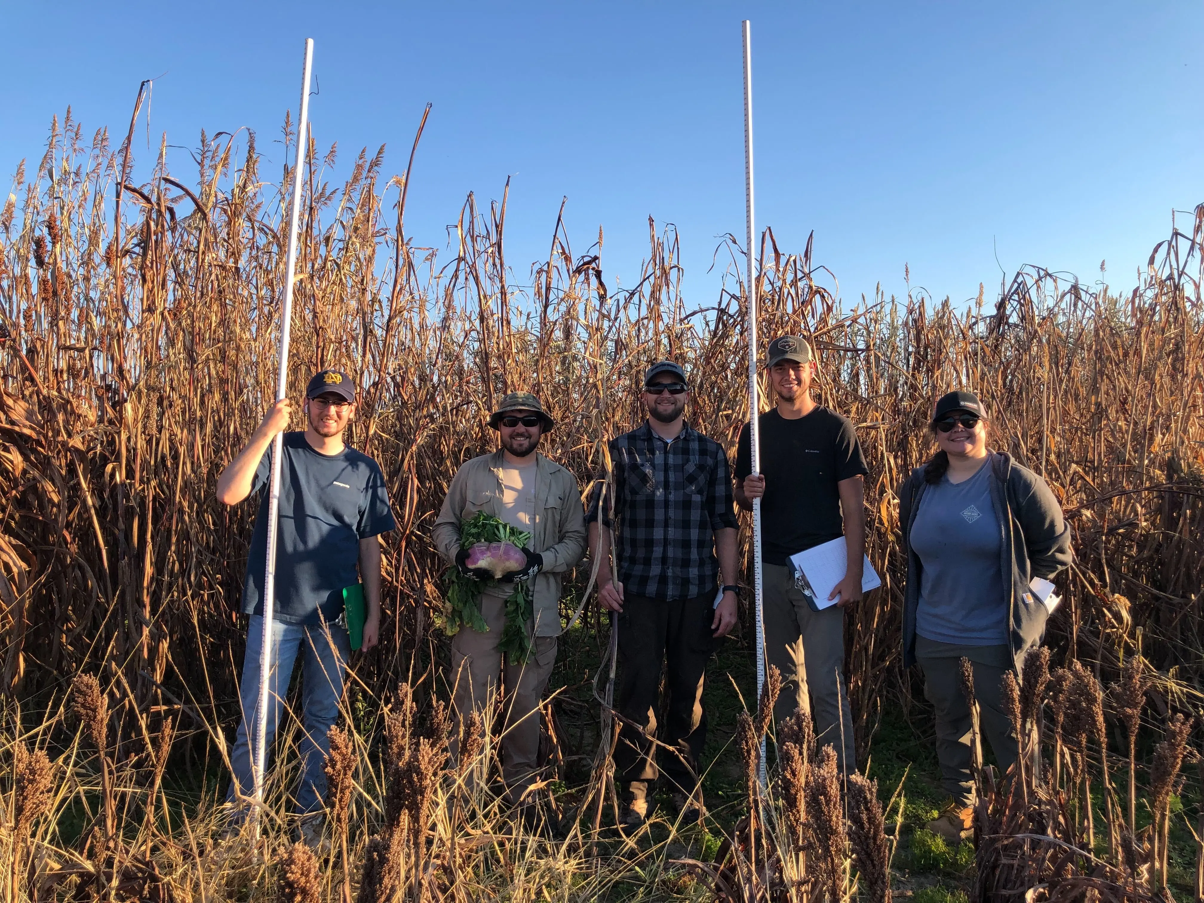
The Lab's Measurements
To support our research, our team also collects detailed data measurements from the field! Our technicians use tools and machines to measure plant traits like height, biomass (how much plant material is produced), photosynthesis activity, soil characteristics, grain quality, and weather conditions such as temperature and rainfall. These measurements are recorded regularly throughout the growing season, from June to October, in every experimental field plot. All the collected values are organized and stored in an excel file, which is part of this project’s dataset, but also what you will be analyzing for this project!
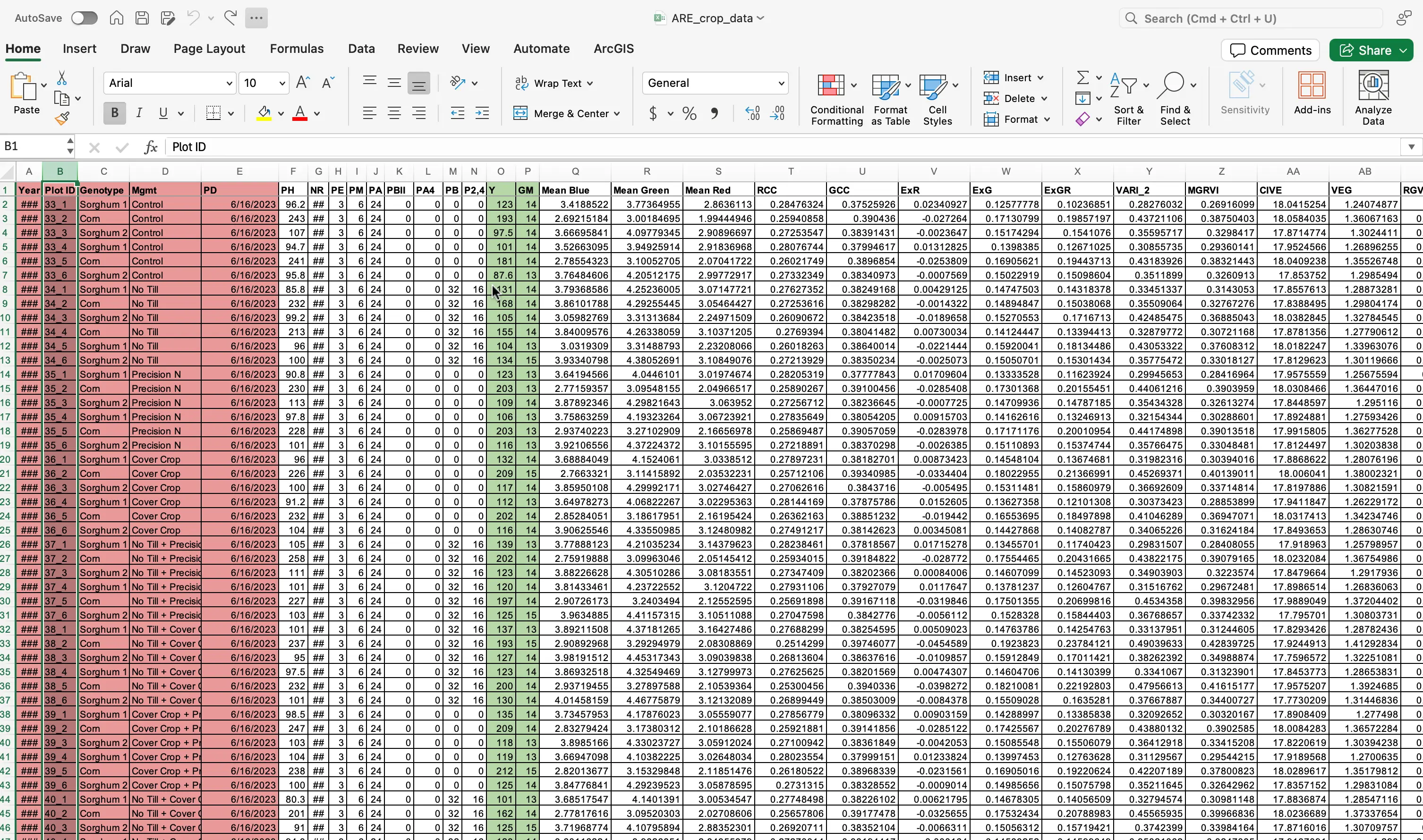
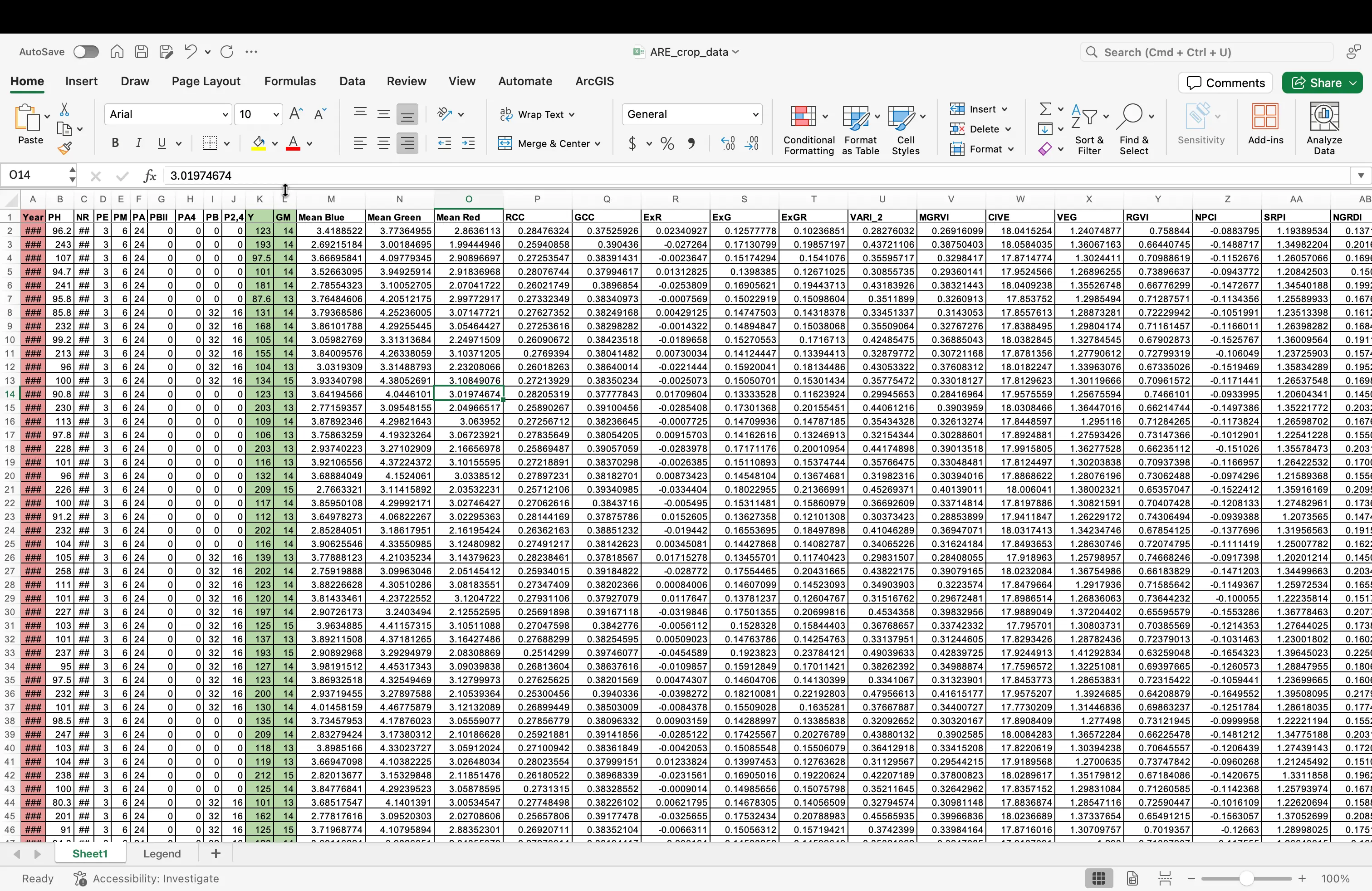
The excel file ARE_crop_data.xlsx is organized with detailed crop data where each row corresponds to a specific plot entry.
- The columns filled in red represent elements related to the field design, such as Year, Plot ID, Genotype, Management Type (Mgmt), and Planting Date (PD)—providing structural and temporal context of the field trial.
- The columns filled in green represent potential target traits used for analysis, including phenotypic measurements like Plant Height (PH), Nutritional Content (e.g., LysP, SC, AMLS), and metabolite or digestibility indicators (e.g., MD_Lys, MD_CF).
- The columns that are white (have no highlighted color), are what is considered potential inputs. They are the different types of data features that could be provided to the model so it can learn patterns and make predictions.
This color-coded structure allows for easy differentiation between experimental setup and measurable outcomes, which is essential for downstream analyses such as Machine Learning-based trait prediction or genotype-performance evaluation.
Please review the following key words for helping you to understand what some of the different target traits mean, or where they are derived from:
- Plant height: The vertical measurement of a plant from the base at soil level to the top of its highest point, often used as an indicator of growth and vigor.
- Biomass: The total mass of living plant material, including stems, leaves, and roots, typically measured to assess growth and productivity, or yield.
- Photosynthesis: Photosynthesis is the biological process by which green plants convert sunlight, carbon dioxide, and water into energy-rich sugars and oxygen. This light-driven conversion occurs primarily through chlorophyll pigments, which capture and absorb light energy. The efficiency of this process, especially within Photosystem II, is quantified by the quantum yield of PSII (ΦPSII or PhiPS2), which indicates the proportion of absorbed light effectively used in photochemical reactions. Chlorophyll content is thus a key factor influencing both light absorption and overall photosynthetic performance.
- Soil characteristics: The physical, chemical, and biological properties of soil—such as texture, pH, moisture, and nutrient content—that influence plant growth.
- Grain quality: The set of traits in harvested grain—including size, weight, nutritional content- such as crude protein, amylose, lysine, crude fat, and purity—that determine its market value and suitability for consumption or processing.
- Genotype-performance evaluation: The assessment of how different plant genotypes perform under specific environmental or management conditions, often based on traits like yield, stress tolerance, and growth rate.
With these key terms being defined should help your understanding of the ideas behind target traits picked for analysis.
Your Key Objective
The objective of the machine learning activities is to develop a model to predict a plant trait (such as yield, seed protein content, chlorophyll a fluorescence, etc.) from diverse data collected by drone, physiological instruments, and technicians in the field, along with climate data. This will help you gain modeling and machine learning skills. Below are the instructions to help you accomplish these tasks.

Before You Begin
In this module, we will be using the Google Colab online coding environment we created during the Installation steps. If you have not done these steps or need a refresher, please refer back to the Installation Guide for details on setting up a Google Colab online environment.
Instructor's Notes
Timing: The entirety of Part 1 fits in roughly 1 - 2 hours of lecture content, depending on how quickly students digest the material.
Tech Prep: Ensure students have Google accounts; test Colab access beforehand.
Differentiation: Provide a cleaned dataset in case students struggle with Excel.
Setting Up Your Project
Download Project Files
- Your team will be accessing the files you need to begin this module here: Project Files.
- You will be looking for the folder labeled Section2: Machine_Learning_Regression_Models.
- Double click this folder, and you should now see two files:
ARE_ML_code.ipynb&ARE_crop_data.xlsx. - You are now going to want to save both of these files, individually, to your local computer. We recommend saving them in the same place as one another. To save a file from Google Drive, find the 3 dots, and click them. You should see a button to
Download.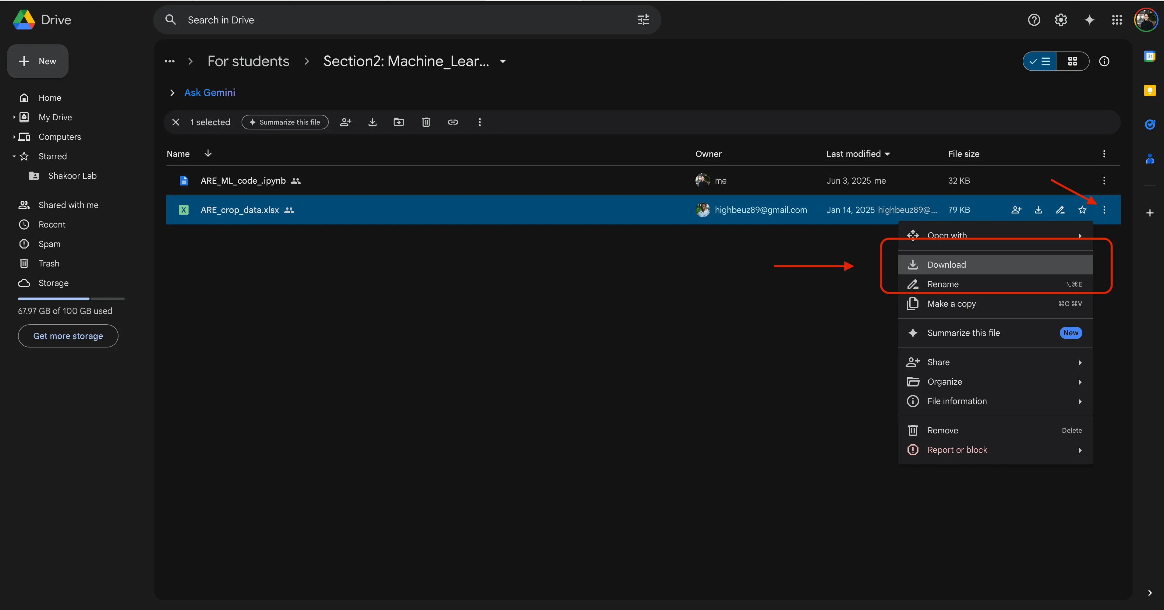
- When prompted, select your file location of choice to place the files on your computer.
- You now have two downloaded files. In the
ARE_crop_data.xlsxfile, you will find the data collected throughout the field season. This is what will be our dataset. Within theARE_ML_code.ipynbfile, you are going to see 6 large code blocks. These blocks hold code for 6 different machine learning models, in which you are to use with the excel dataset file for analysis.
Meet the Dataset
We gave you an Excel file called ARE_crop_data.xlsx.
Each row = one plot in the field.
Each column = one piece of information we measured.
| Column Color | What it means | Example columns |
|---|---|---|
| Red | Field setup | Year, Plot ID, Genotype |
| Green | Plant traits | Plant Height (PH), Yield (Y), Protein Crude (PC) |
Student Task
Student Task A: Explore
Open the spreadsheet and answer →
How many rows are there in total?
Name a few green columns that look interesting to you.
Pause & Discuss
Students: Take 10 minutes to jot down:
- One reason scientists use machine learning.
- One green-column trait you might want to predict.
Teachers: Quick check-for-understanding—call on a few pairs to share.
- Any confusion about red vs. green columns?
- Does everyone have both files downloaded?
Give a thumbs up/sideways/down on: “I know what my dataset rows and columns represent.”
SECTION 2
In this section, we will discuss picking your target traiting and cleaning your data to make it usable!
ML Model Overview
As mentioned in the previous section, in the ARE_ML_code.ipynb file, you will see provided code that implements six regression models to handle crop trait prediction. Please see the following to see what these models are called, and a very high level summary of each of them:
- Partial Least Squares (PLS) Regression: Finds patterns by combining features into simpler parts to predict something when you have lots of related data.
- Lasso Regression: Helps pick only the most important features by shrinking less useful ones down to zero.
- ElasticNet Regression: Combines Lasso and another method (Ridge) to balance feature selection and avoid overfitting.
- Bayesian Ridge Regression: Adds a bit of randomness to the prediction process to make it more stable and handle uncertainty better.
- Xtreme Gradient Boosting (XGBoost): Builds lots of small decision trees that learn from each other to make powerful predictions.
- Support Vector Regression (SVR): Tries to find a smooth line that fits the data while ignoring small errors, making it good for tricky patterns.
You should know!
Regression is a way of finding a pattern in data so we can make predictions. Imagine you plot a bunch of points on a graph. Maybe each point shows how many hours a student studied and what score they earned. The points might not line up perfectly, but regression finds the best-fitting line (or curve) that goes through the “middle” of the points. Once we have that line, we can use it to predict what score someone might get if we know how many hours they study. In short: regression looks at past data, finds a trend, and uses that trend to make smart predictions.
You will have access to each of these, so feel free to use any of them or implement additional models such as Random Forest or Linear Regression, depending on your preference and familiarity.
Here is another way to view these models, in more simple terms:
| Model | One-line idea | When it shines |
|---|---|---|
| PLS | Combines many related features into simpler parts | Tons of similar columns |
| Lasso | Shrinks useless features to zero | You suspect only a handful of columns matter |
| ElasticNet | Mix of Lasso + Ridge | Balanced approach |
| Bayesian Ridge | Adds uncertainty estimates | Noisy data |
| XGBoost | Many small decision trees that learn from mistakes | Complex, non-linear patterns |
| SVR | Finds the best-fit line while ignoring small errors | Medium-sized datasets |
You should know!
For this portion of the activity, we have provided all of the code you will need, for you! No prior coding experience needed!
Choosing Your Target Trait
In machine learning, especially in predictive modeling, we try to predict something based on other pieces of information. That "something" we want to predict is called the target trait (also known as the target variable or label). In this project, the traits in your dataset are measurable characteristics of the plants—such as Yield (Y), Protein Crude (PC), or Quantum Yield of PSII (PhiPS2).
Everyday Example:
Imagine you’re coaching your school’s track team. You want to predict an athlete’s 200‑meter sprint time (target trait) from other measurable facts, such as their 100‑meter time, vertical jump height, and average weekly training hours (input features). The computer would learn the relationship between those inputs and the sprint time, just like we’ll do with plant traits!
You will choose one of these green-highlighted traits as your target trait. This is the outcome your model will try to predict. For example, if you choose "Yield (Y)" as your target, the goal of your machine learning model will be to predict how much yield a plant will produce based on the values of other traits.
The other traits in the dataset, such as plant height, chlorophyll content, or leaf area, will serve as your input features. These features are the information the model uses to make predictions about the target trait. The better the quality and relevance of your input features, the more accurate your model’s predictions will be.
Before training your model, you’ll need to do some cleaning of the dataset! This means that in the next steps coming up, we will be removing:
- Non-numeric columns, like
plant IDornotes - Irrelevant data, such as field layout info or metadata not useful for prediction
Your cleaned dataset should contain only numeric columns related to plant traits, one of which will be your target, and the rest will be your inputs.
In summary, you will select one trait to predict (referred to as the “target”) from among the green-filled traits (e.g., Yield (Y), protein crude (PC), or quantum yield of PSII (PhiPS2)), while using other available traits as input features. Make sure to remove any non-numeric or irrelevant columns (like the field design columns mentioned above) before proceeding!
Key Terms to Remember:
- Trait: Any measurable characteristic of the plant.
- Target trait (target variable): The trait you are trying to predict (e.g., Y, PC, or PhiPS2).
- Input features (predictors): The traits used to help predict the target.
Student Task
Student Task B: Brainstorm
With the
ARE_crop_data.xlsxfile open, choose a possible target trait other than yield that a plant scientist might find useful (e.g. Protein Crude).Write down at least four input features you think could help predict it.
For each feature, write one sentence explaining why it might influence the target trait (You may have to look some of them up using our glossary or the internet).
Let us resume where we have left off! As a recap, you should have the following two files downloaded to your computer: ARE_ML_code.ipynb & ARE_crop_data.xlsx.
We are now going to move on to preparing the dataset you will be working with.
Create a Project Directory (Optional)
This is an optional step. If you already know the path of your downloaded files, you can keep them there, or you can condense them into a folder. The choice is yours!
- Create a folder for your project (e.g.,
geo_ml_project). - Place your dataset (
ARE_crop_data.xlsx) in this folder. - Now place your coding notebook in the same folder (
ARE_ML_code.ipynb). - You now have what is called a Project Directory! This is just a fancy term for a place where you have all code files related to the same project, stored in one spot.
Prepare the Dataset
Let us move on to preparing and cleaning the ARE_crop_data.xlsx dataset.
- Ensure the dataset that you just downloaded is in
.xlsxformat. - Open the file using Excel.
- With the file open, discard the columns related to field design such as
PlotID,Genotype,Mgmt, andPlanting Date (PD).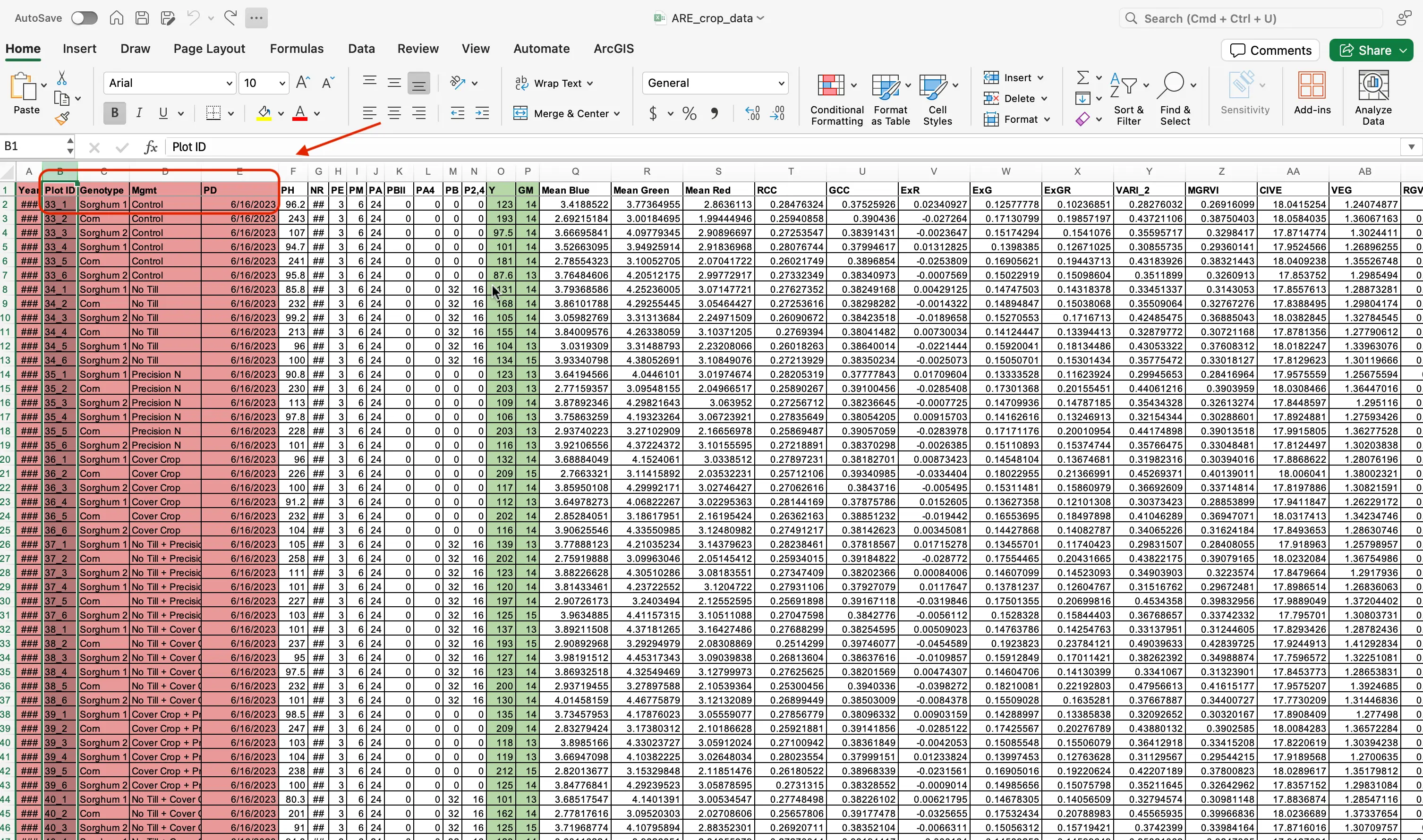
Student Task
Student Task C: Answering Question
- Why might keeping
PlotIDhurt the model?
- With the columns deleted, this is now how your dataset should now look:
- Odds are, you dataset is already set to how we would like it, but in science it is always best to double check! Select everything in your file (clicking the square in the top left of your data table). While in the
Hometab, find on the top menu the Number Formatting dropdown. Click on this, and scroll down toGeneral. SelectGeneral, even if it is already prepopulated in the dropdown.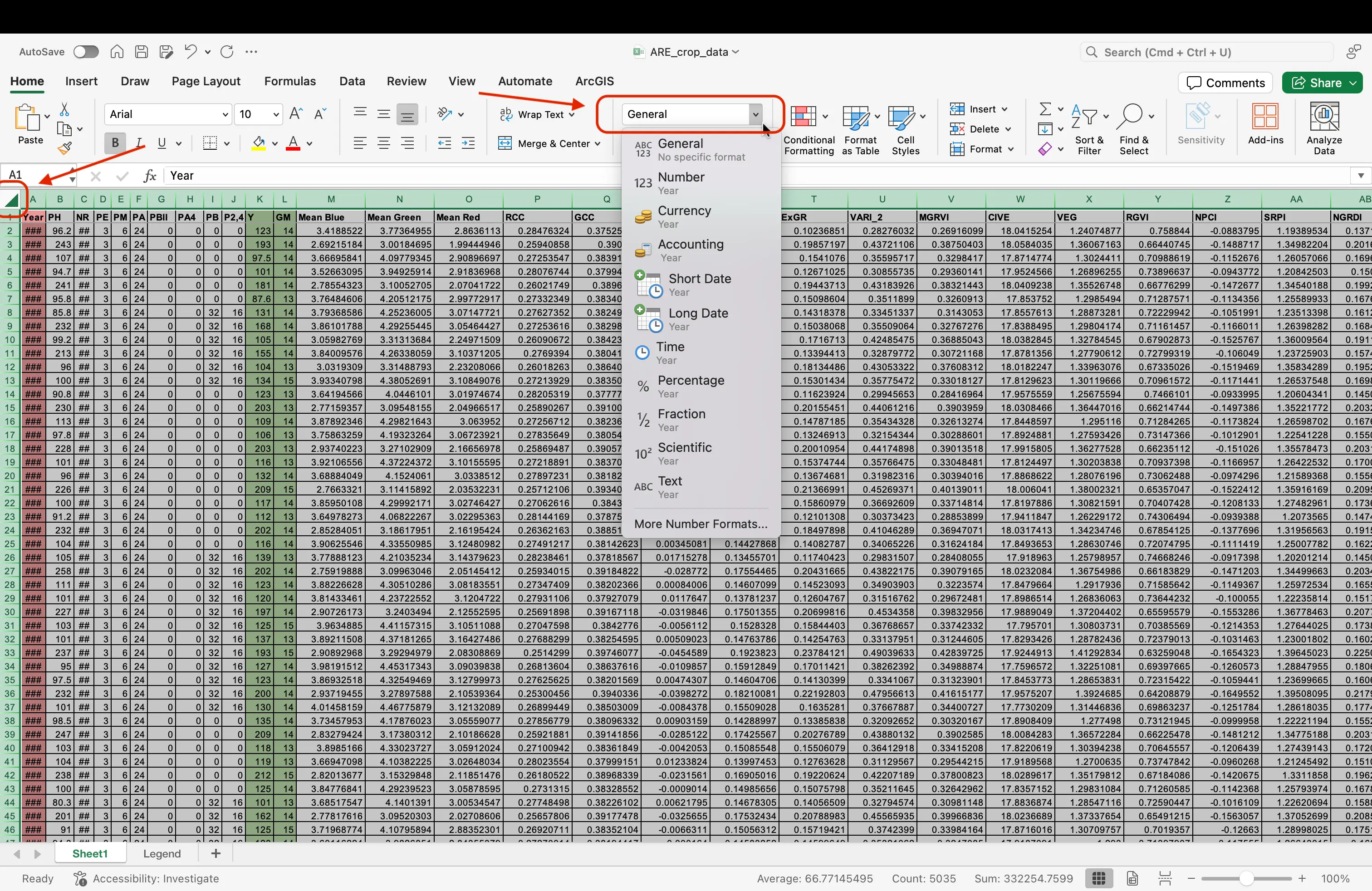
- Your dataset should now look similar this this:
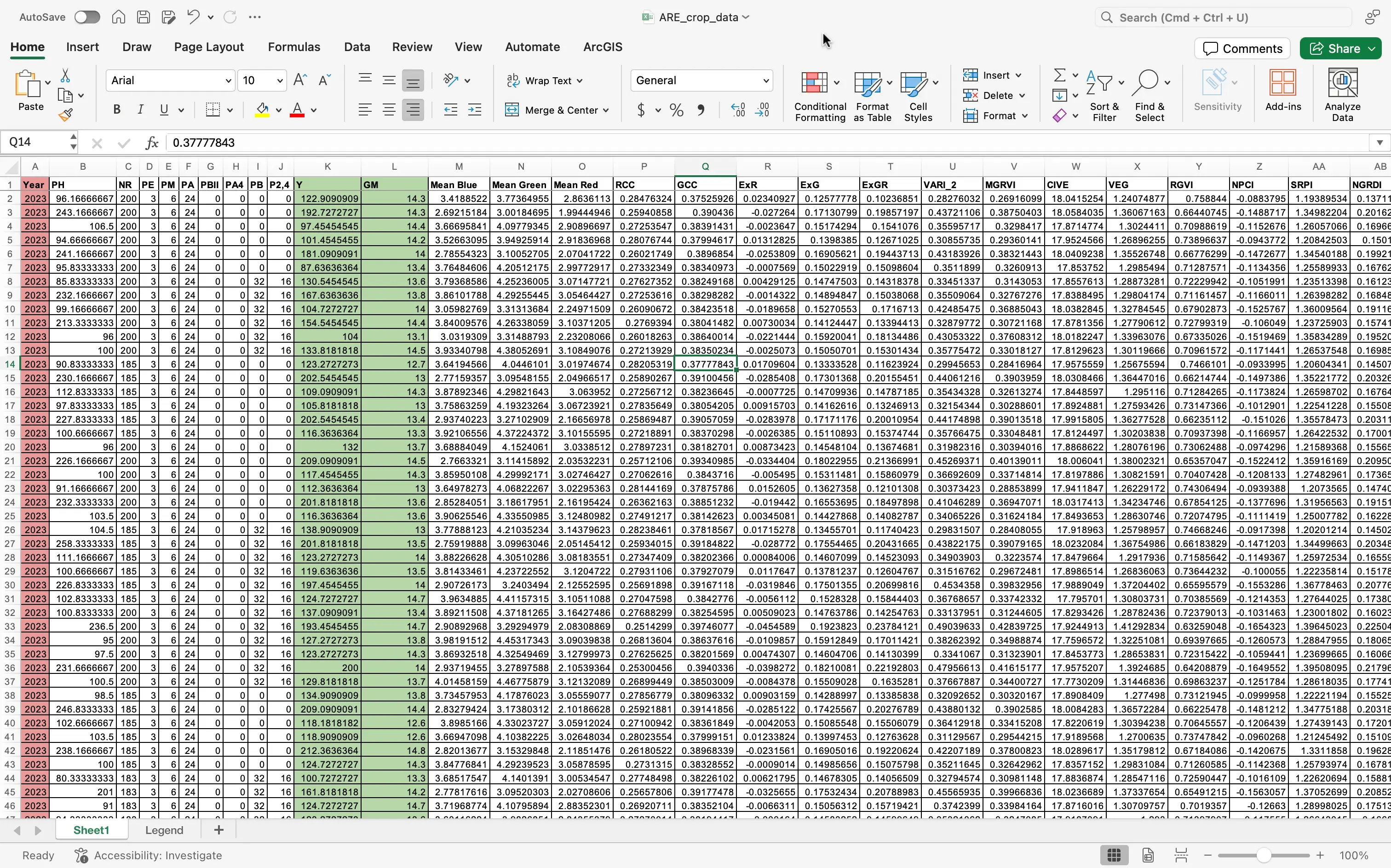
- Make sure to now save your now updated file!
Checkpoint & Questions
Students:
- Circle your chosen target trait in your notes.
- List 3–4 input features you kept, and why.
- Show a partner the columns you deleted. Did you both delete the same ones?
Teachers:
- Ask: “Why is
PlotID(or another ID column) a bad predictor?” - Quick poll: Who changed their mind about a target trait after cleaning?
Take a short stretch/water break before we jump into setting up Google Colab.
SECTION 3
Welcome back! In this section, we will be breaking down the process of moving our code files and cleaned up data to Google Colab, an online code editor!
Moving your files
We are going to now want to move your downloaded project files (or folder if you just combined them), to Google Colab so you can run these files.
With your internet browser open, navigate to the Google Colab website once more, if you are not already there.
Important
If you had the tab open, and did not interact with Google Colab for too long, you may have to restart your runtime to be able to run code again. Remember, this is in the far right corner by clicking the
Connectbutton. You are looking for the green check mark to know you are successfully connected.With Google Colab open, navigate to the Toolbar and select the
Filebutton, and when shown more options, please select theUpload notebookbutton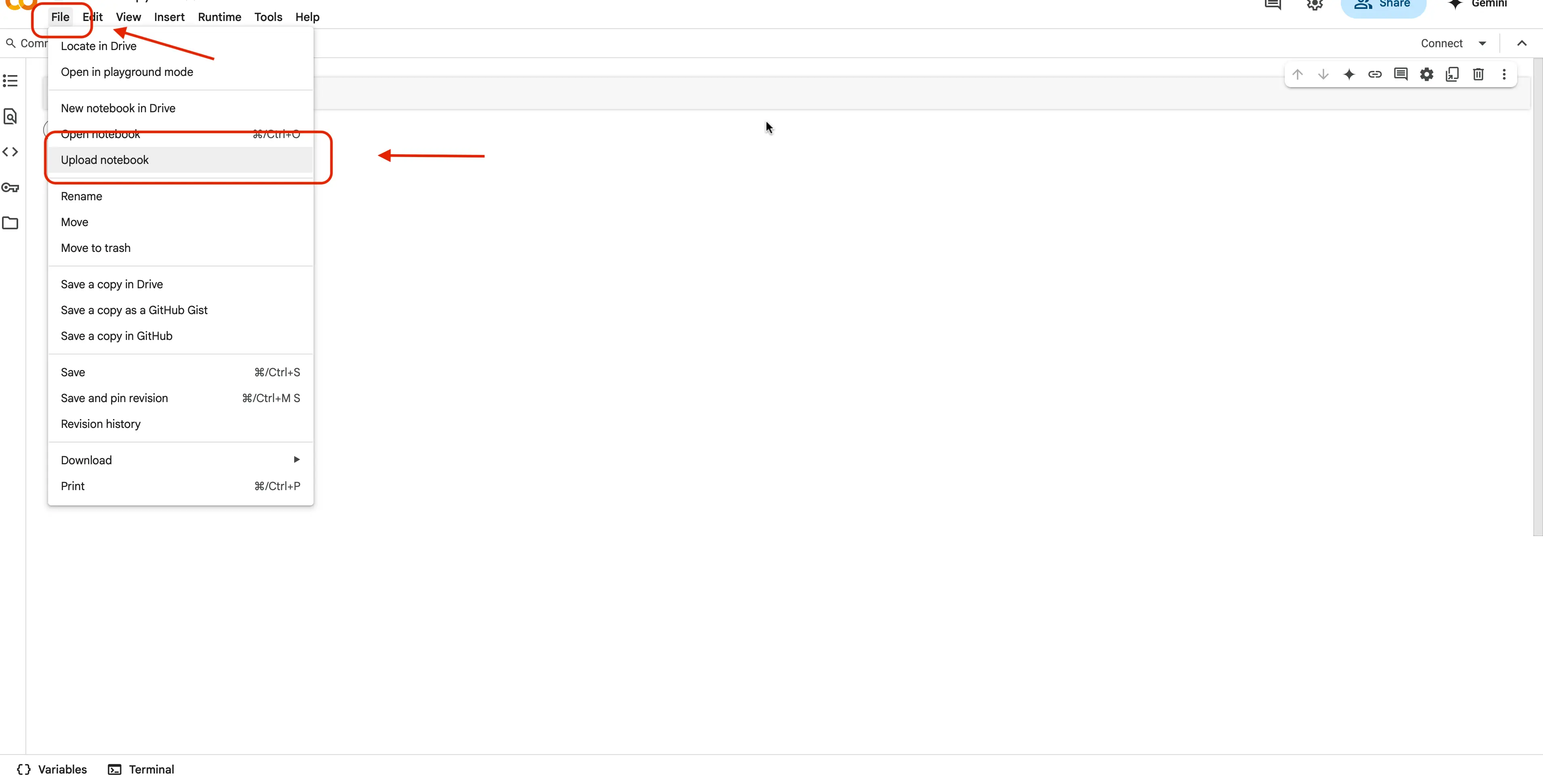
You should now see the Browse button. Click this and navigate to where your
ARE_ML_code.ipynbnotebook file is located.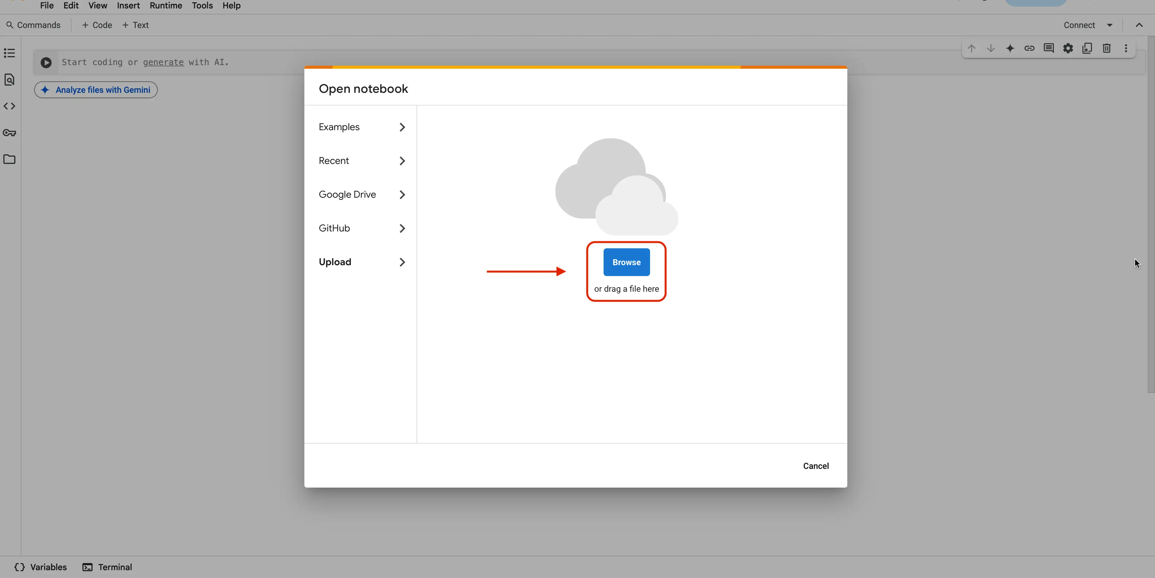
Select the file, and click the
Uploadbutton. This will upload our notebook to Google Colab to be used.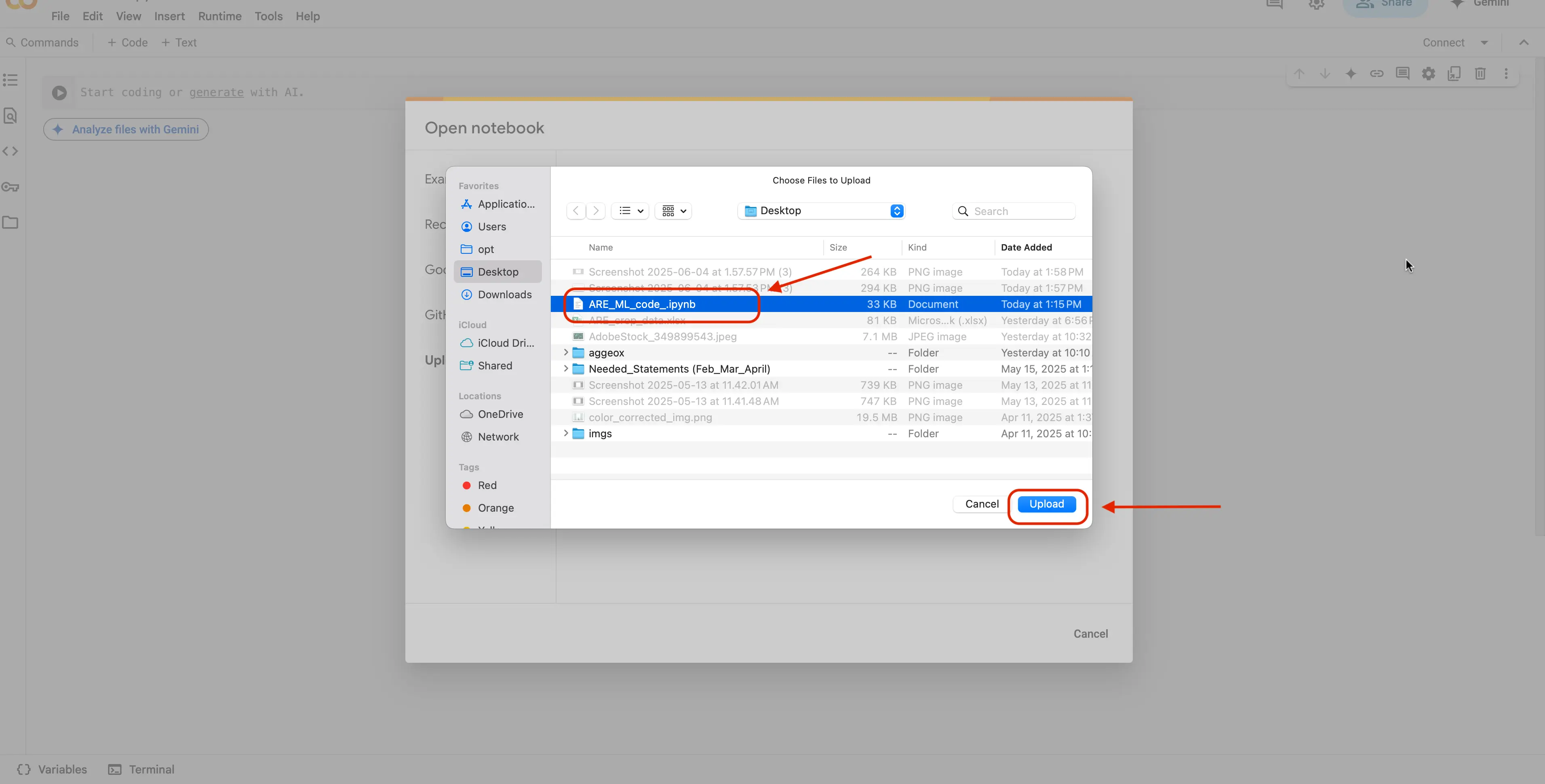
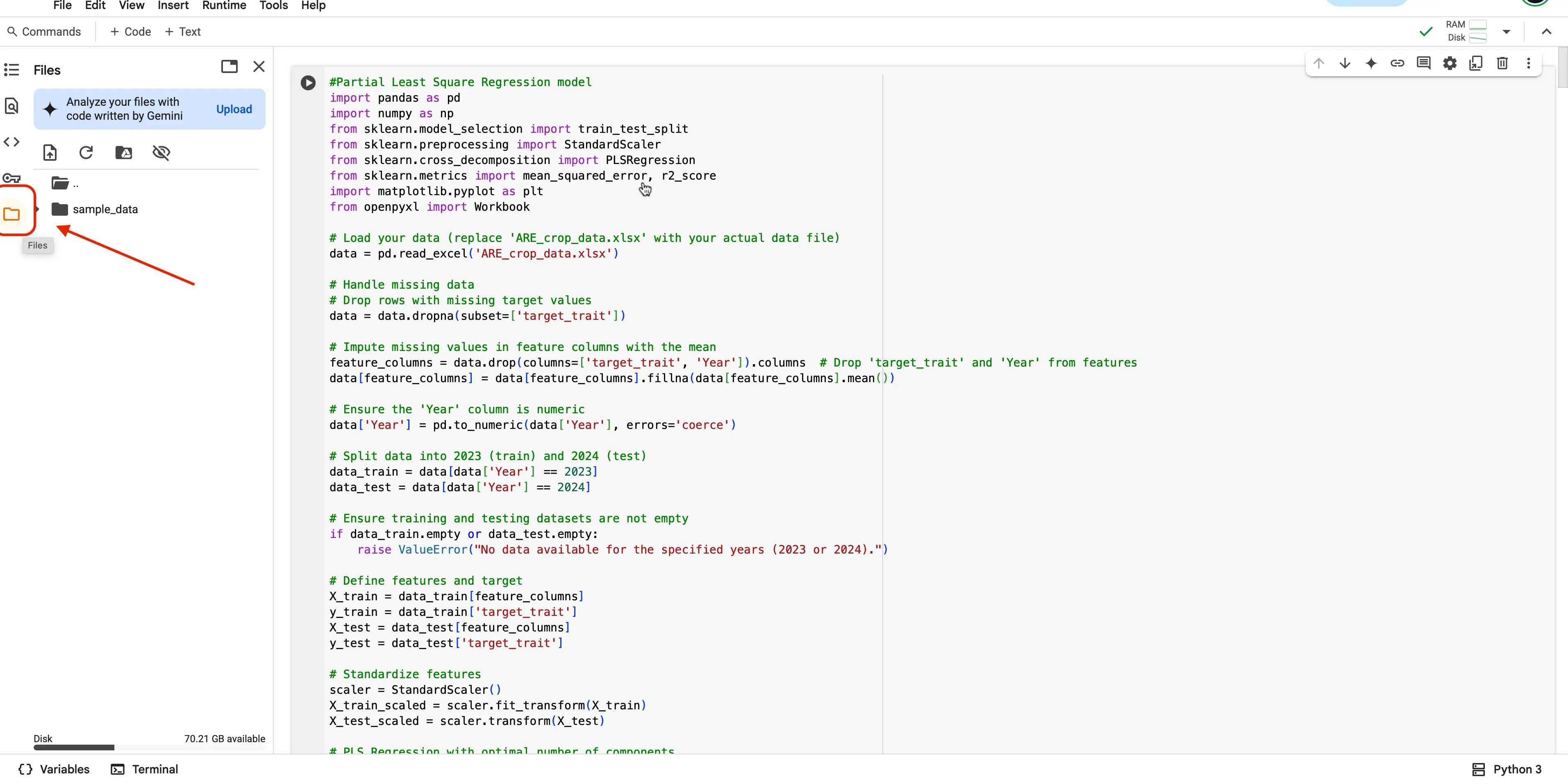
With your file now open, you will now want to navigate to the left side of your screen. You should see 5 icons. You are going to want to click the icon like looks like a folder.
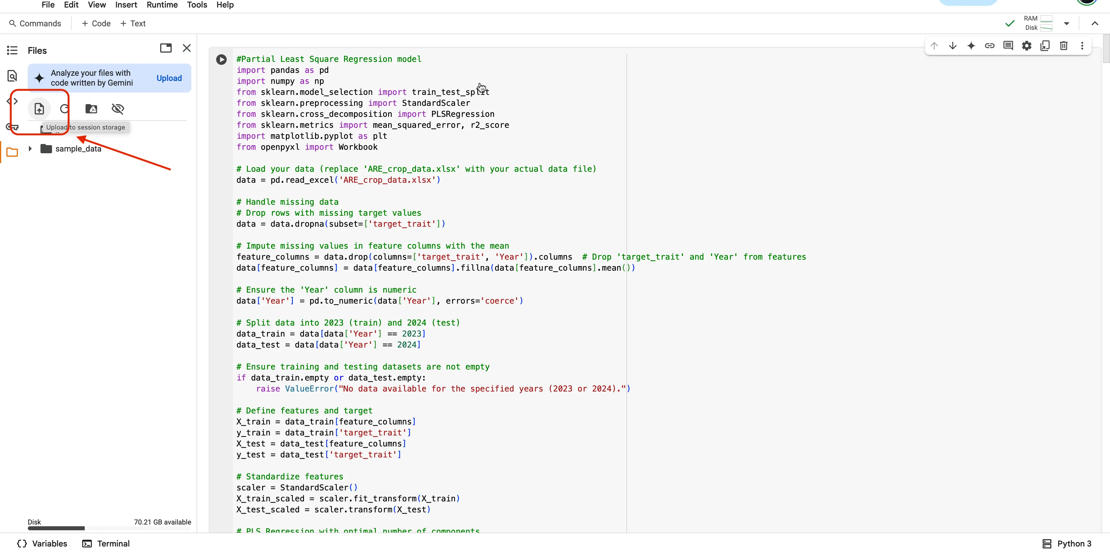
When this tab opens, you will now see 4 more icons. You are going to want to click the first icon, to upload your files.
Your computer should now be prompting you to select from your computer's files. You are going to want to navigate to where you placed the
ARE_crop_data.xlsxdataset file.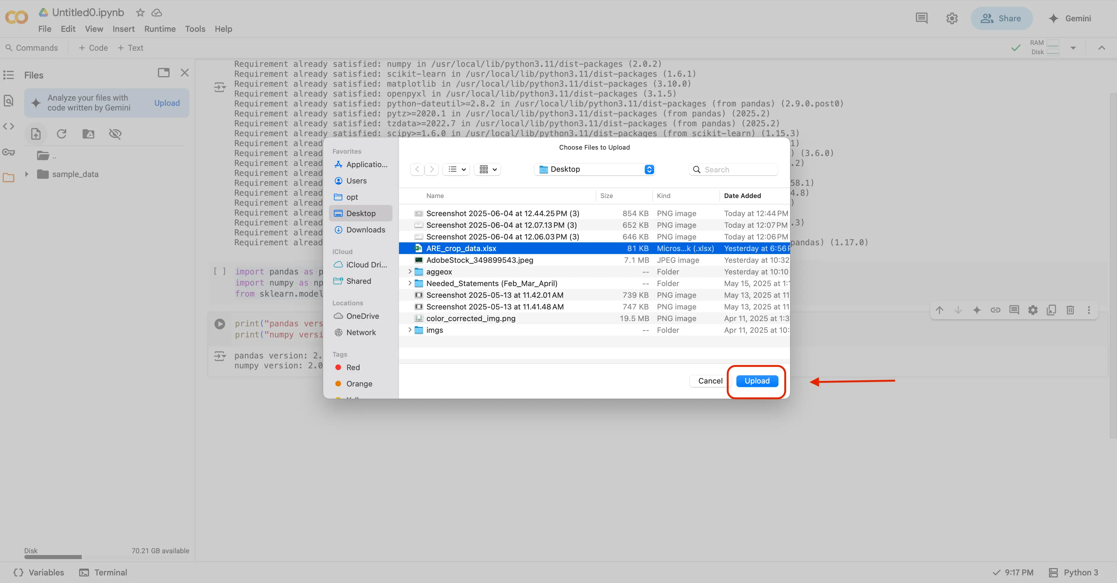
If that was successful, you should now see your file that you selected, in the file selection area in Google Colab.
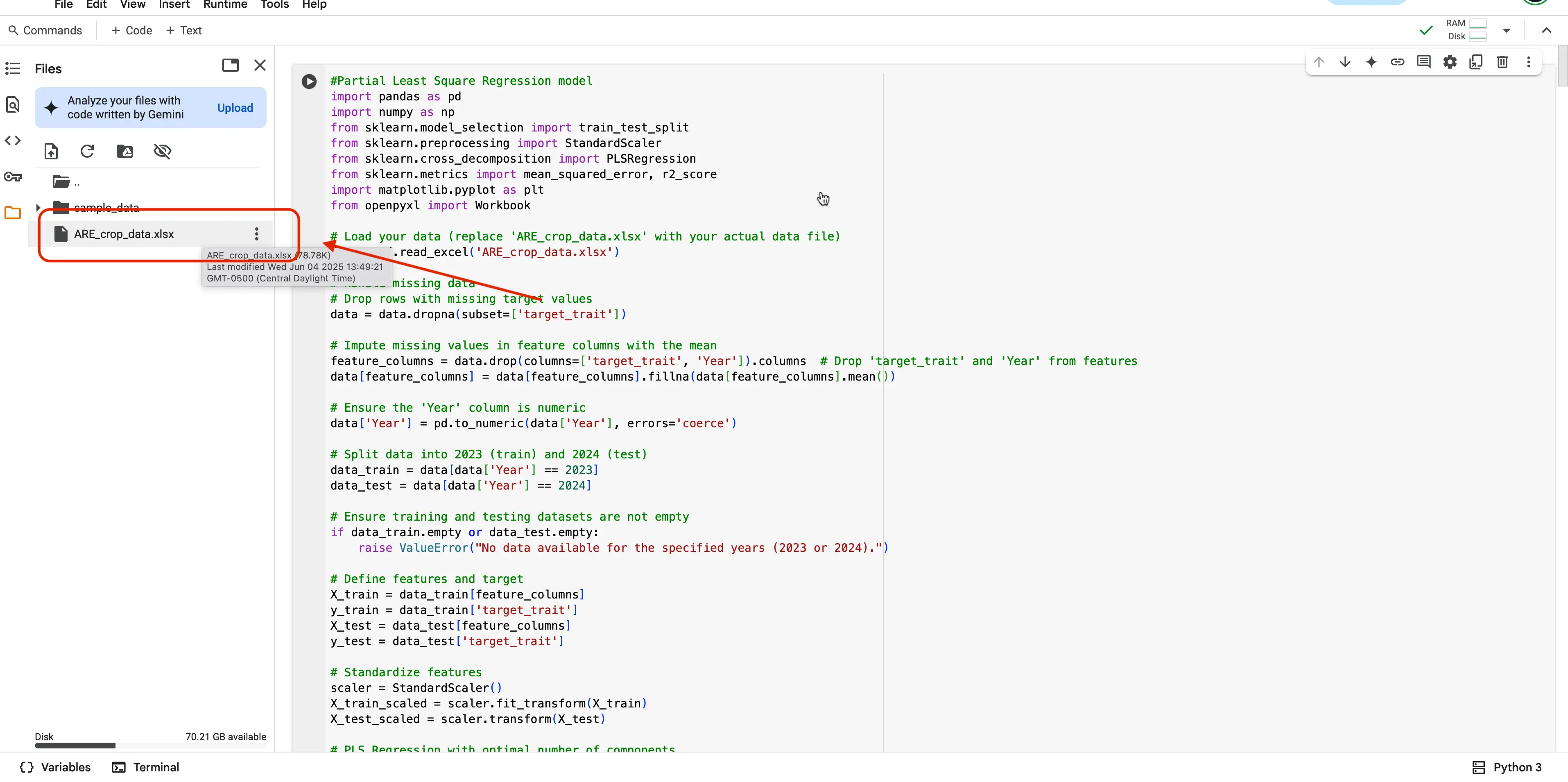
Congrats! Your dataset file is now usable in Google Colab.
You should know!
Whenever you see a # in the code, you should know this means that all of the words following that symbol, represent a comment. In coding, comments are used to explain what the block of code underneath the comment does, or how the code operates. Before running the code, take a few minutes to read through the comments we have provided to you in the code, to get a better understanding of what each block of code is doing!
Depending on your code editor, sometimes comments display as green text, and sometimes they display as gray text. In our code, you are looking for the green text.
Learning Checkpoint
Pop Quiz 🚀
Multiple Choice: Which file contains the code for the machine‑learning models?A. ARE_crop_data.xlsx B. ARE_ML_code.ipynb C. Geo_ml_project
True or False: Genotype is a good input feature to keep for model training.
Fill in the Blank: In the spreadsheet, the color green marks **____**.
Multiple Choice: You chose Protein Crude (PC) as your target trait. Which of the following would NOT be a helpful input feature?A. Plant Height B. Rainfall C. File Name
Short Answer: Why should non‑numeric columns be removed before training a regression model?
Answers
SECTION 4
Learning Continued
At this point, you might be thinking...
Alright, but what’s the point of all this? Why do we even bother with modeling and regression models in the first place?
We had the very same questions when we started out, so we took the time to reflect on our journey, pinpoint the most pressing questions we had, and put together clear, straightforward answers to help you make sense of it too!
What is Modeling? Modeling is the process of creating a simplified version of real-world scenarios using mathematics and data. In science, we use models to understand patterns, make predictions, and test ideas without always needing to run experiments in real life.
What is a regression model? A regression model is a type of statistical or machine learning model used to understand and quantify the relationship between one or more input variables (called independent variables or features) and a continuous output variable (called the dependent variable or target).
Why Use Models? Imagine trying to predict crop yield, weather, or even how a disease spreads — it's too complex to guess! Modeling helps us:
- Predict outcomes
- Save time and resources by running simulations
- Understand hidden relationships between many factors (like sunlight, water, nutrients)
What was the Model Doing? A model takes data from input features (e.g., plant height) and learns from these data to predict an outcome — such as grain nutritional quality (amylose, protein or starch content). Behind the scenes, the model is doing lots of math to find patterns and make the best possible guesses.
How Do We Interpret the Model? Once the model makes predictions, we compare the prediction data to actual data collected by the scientists in the field to see:
- How close was the prediction to the field data? → Good model
- How far off was it from the field data? → Maybe we need more data or a better model
How do we test the accuracy of Models?
R² (Coefficient of determination R-squared) – Tells us how well the model fits the real data (0 indicates the model explains none of the variability whereas 1 indicates that all of the variability is explained by the model)
RMSE (Root Mean Squared Error) – Measures the average difference of the actual data points from the predicted values . A value of zero indicates a perfect fit, while higher values indicate more error and less precise predictions.
What are the predictors variables? When you integrate diverse data as inputs in models, not all the variables will be relevant to the model to make good guesses. Then the most important variables or features are crucial information to understand which variable drives the model output, then next time you will not need to collect all the other data.
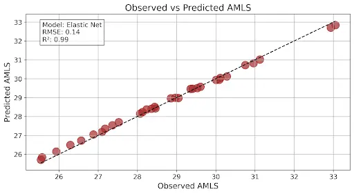
What is an example of expected regression plots? Here is an example of regression plots you might expect to generate. This graph that you are seeing has very good model output as the R2 is close to 1 and the RMSE is low:
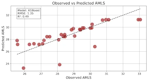
This graph shows a good model output as R2 is a midpoint between 0 and 1 and the RMSE is higher than what the above graph is showing:
Stop for a breath!
Take a minute to reflect on all of the information. We know it is a lot to take in at once! Machine Learning is not an easy concept, it takes a long time to understand well and become an expert at. If you are curious and eager to learn more, please see the links below to become an expert yourself!
If the above definitions are a bit much to digest at the moment, please see the table below that breaks the vocabulary down to simpler terms, and gives an everyday example:
| Concept | What it Means | Everyday Example |
|---|---|---|
| Modeling | Building a simplified version of the real world so we can test ideas quickly. | A paper-airplane prototype lets you test wing shapes before building a real glider. |
| Regression Model | A math recipe that links one or more inputs to a number you care about. | Using hours-studied to guess your math-test score. |
| Why Use Models? | They help us predict, save time, and spot hidden patterns. | Weather apps predict rain so you know to grab an umbrella. |
| What the Model Is Doing | It learns the relationship between inputs and the target from examples. | A computer learns how pizza size relates to price, then guesses the cost of a new pizza. |
| Interpreting the Model | We compare its guesses to real data to judge quality. | If your step-counter app says you walked 9,950 steps but your watch shows 10,000, that’s pretty close—good model! |
| R² (Coefficient of Determination) | Tells us what fraction of the real-world variation the model explains (0–1). | R² = 0.9 means 90 % of house-price differences are explained by size and location—great! |
| RMSE (Root Mean Squared Error) | Average size of the model’s mistakes (lower = better). | An RMSE of 3 °F means a forecast is off by ~3 °F on average. |
| Predictor Variables (Input Features) | The pieces of information the model uses. | Predicting fuel efficiency from car weight and engine size (but not paint color). |
| Regression Plot | A scatterplot of Predicted vs. Actual values to visualize performance. | If dots for predicting class heights hug the diagonal line, your height-model rocks. |
Learning Resources
Want to learn more? Checkout these links here!
Please visit this source if you want to learn more about the different types of machine learning: Five Machine Learning Types to Know
Find out here how others are using machine learning in agriculture! Machine Learning in Agriculture: Use Cases and Applications
If you want to read more about how machine learning may benefit agriculture, visit this resource: What is Machine Learning & How Will it Benefit Agriculture?
Glossary
Identified Keywords
- Plant height
- Biomass
- Photosynthesis
- Soil characteristics
- Grain quality
- Genotype-performance evaluation
- Model
- Modeling
- Learning models
- Regression
- Observed and predicted values
- Prediction
- Machine learning
- Plant trait
- Target trait
- Input features
- Trait prediction
- Training a model
- R2
- RMSE
- Adjusting model parameters
- Model accuracy
- Cross-validation
- Grid search
- Randomized search
- Hyperparameter
- Loss curves
- Accuracy metrics
- Feature importance
Definitions
Plant height: The vertical measurement of a plant from the base at soil level to the top of its highest point, often used as an indicator of growth and vigor.
Biomass: The total mass of living plant material, including stems, leaves, and roots, typically measured to assess growth and productivity, or yield.
Photosynthesis: Photosynthesis is the biological process by which green plants convert sunlight, carbon dioxide, and water into energy-rich sugars and oxygen. This light-driven conversion occurs primarily through chlorophyll pigments, which capture and absorb light energy. The efficiency of this process, especially within Photosystem II, is quantified by the quantum yield of PSII (ΦPSII or PhiPS2), which indicates the proportion of absorbed light effectively used in photochemical reactions. Chlorophyll content is thus a key factor influencing both light absorption and overall photosynthetic performance.
Soil characteristics: The physical, chemical, and biological properties of soil—such as texture, pH, moisture, and nutrient content—that influence plant growth.
Grain quality: The set of traits in harvested grain—including size, weight, nutritional content- such as crude protein, amylose, lysine, crude fat, and purity—that determine its market value and suitability for consumption or processing.
Genotype-performance evaluation: The assessment of how different plant genotypes perform under specific environmental or management conditions, often based on traits like yield, stress tolerance, and growth rate.
Model: An abstract representation or mathematical function that maps input data to output predictions based on learned patterns from data.
Modeling: The process of creating and refining a model by selecting its form, structure, and parameters to best capture relationships in data.
Learning models: A category of models in which parameters are automatically inferred from data through algorithms, as opposed to being manually specified (e.g., linear regression, decision trees, neural networks).
Regression: A type of supervised learning task and statistical method focused on modeling the relationship between one or more input variables and a continuous output variable.
Observed and predicted values:
- Observed values: The actual, measured outcomes in the dataset (ground truth).
- Predicted values: The outputs generated by the model when given input features.
Prediction: The act of using a trained model to estimate the output (target) for new, unseen input data.
Machine learning: A field of computer science that develops algorithms and models which improve their performance on a task through experience (i.e., by learning from data).
Plant trait: A measurable characteristic of a plant (e.g., leaf area, height, biomass) used in biology or agronomy studies.
Target trait: The specific plant trait that a model is trained to predict (sometimes called the dependent variable).
Input features: The set of variables (independent variables) used by a model as inputs to predict the target trait (e.g., spectral indices, environmental measurements).
Trait prediction: The task of estimating a plant’s target trait value using a model and a set of input features.
Training a model: The process of feeding input–output pairs (features and observed target values) into a learning algorithm so that the model’s parameters are adjusted to minimize prediction error.
R² (Coefficient of Determination): A metric that indicates the proportion of variance in the observed target values explained by the model; ranges from 0 to 1, with higher values indicating a better fit.
RMSE (Root Mean Squared Error): A metric that quantifies the average magnitude of prediction errors by taking the square root of the average squared differences between observed and predicted values.
Adjusting model parameters: The act of modifying either model weights (in learning algorithms) or structural settings to improve performance; often refers to both training (learning weights) and tuning (hyperparameter selection).
Model accuracy: A general term for metrics that evaluate how well a model’s predictions match the true values; in regression contexts, this often involves R², RMSE, MAE, etc.
Cross-validation: A technique for assessing model performance by partitioning data into multiple subsets (folds), training on some folds, and validating on the remaining fold(s) to estimate how well the model generalizes.
Grid search: A systematic approach to hyperparameter tuning where a predefined set of hyperparameter values is exhaustively evaluated to find the combination that yields the best model performance.
Randomized search: An alternative hyperparameter tuning method that samples a fixed number of hyperparameter combinations at random from a specified distribution, often more efficient than grid search when the search space is large.
Hyperparameter: A configuration setting for a learning algorithm or model (e.g., learning rate, regularization strength, number of hidden layers) that is set before training begins and not learned directly from the data.
Loss curves: Plots showing how the model’s loss (error) changes over training iterations or epochs, used to diagnose underfitting, overfitting, and convergence behavior.
Accuracy metrics: Quantitative measures (e.g., R², RMSE, MAE for regression; accuracy, precision, recall for classification) that evaluate a model’s performance against ground truth.
Feature importance: A ranking or score indicating how much each input feature contributes to the model’s predictions, often computed using methods like permutation importance, tree-based importance scores, or SHAP values.
Next up
In Part 2, we will begin running the model, understanding the results, and then finally tuning the model to achieve even more accurate results! If you wish to learn more, please continue to read through the Learning Continued section below. Once you are finished, head on over to the next part of the activity!